Regression Discontinuity Design
Goal of today
We replicate Liu et al (2024) that study judicial reforms and strategic sentencing in autocracies. The full replication materials can be found here.
Load necessary packages
rm(list=ls())
library(haven)
library(rdrobust)
library(rddensity)
library(ggplot2)
library(ggeffects)
library(dplyr)
library(scales)
library(stargazer)
library(fastDummies)
library(sjPlot)
library(fixest)
library(sjmisc)
Load data
trial<- read_dta("trial_replication.dta") #Load the full data
civilian<-trial[trial$category_e==0,] #The data including only civilian defendants
Show all package versions
utils:::print.sessionInfo(sessionInfo()[-8],locale = FALSE)## R version 4.4.1 (2024-06-14)
## Platform: aarch64-apple-darwin20
## Running under: macOS 15.6.1
##
## Matrix products: default
## BLAS: /Library/Frameworks/R.framework/Versions/4.4-arm64/Resources/lib/libRblas.0.dylib
## LAPACK: /Library/Frameworks/R.framework/Versions/4.4-arm64/Resources/lib/libRlapack.dylib; LAPACK version 3.12.0
##
## attached base packages:
## NULL
##
## other attached packages:
## [1] sjmisc_2.8.9 fixest_0.12.1 sjPlot_2.8.15 fastDummies_1.7.4
## [5] stargazer_5.2.3 scales_1.4.0 dplyr_1.1.4 ggeffects_1.5.2
## [9] ggplot2_4.0.0 rddensity_2.5 rdrobust_2.2 haven_2.5.4
##
## loaded via a namespace (and not attached):
## [1] gtable_0.3.6 lpdensity_2.4 xfun_0.49
## [4] bslib_0.8.0 bayestestR_0.13.2 insight_0.20.4
## [7] lattice_0.22-6 tzdb_0.4.0 numDeriv_2016.8-1.1
## [10] vctrs_0.6.5 tools_4.4.1 sjstats_0.18.2
## [13] generics_0.1.4 sandwich_3.1-1 tibble_3.3.0
## [16] pkgconfig_2.0.3 Matrix_1.7-0 RColorBrewer_1.1-3
## [19] stringmagic_1.1.2 S7_0.2.0 lifecycle_1.0.4
## [22] compiler_4.4.1 farver_2.1.2 codetools_0.2-20
## [25] htmltools_0.5.8.1 sass_0.4.9 yaml_2.3.10
## [28] Formula_1.2-5 nloptr_2.1.1 pillar_1.11.1
## [31] jquerylib_0.1.4 tidyr_1.3.1 MASS_7.3-60.2
## [34] cachem_1.1.0 boot_1.3-30 multcomp_1.4-26
## [37] nlme_3.1-164 tidyselect_1.2.1 sjlabelled_1.2.0
## [40] digest_0.6.37 performance_0.11.0 mvtnorm_1.3-3
## [43] purrr_1.1.0 bookdown_0.40 forcats_1.0.0
## [46] splines_4.4.1 fastmap_1.2.0 grid_4.4.1
## [49] cli_3.6.5 magrittr_2.0.4 survival_3.6-4
## [52] TH.data_1.1-2 broom_1.0.7 readr_2.1.5
## [55] dreamerr_1.4.0 withr_3.0.2 backports_1.5.0
## [58] estimability_1.5.1 modelr_0.1.11 rmarkdown_2.29
## [61] emmeans_1.10.1 lme4_1.1-35.5 blogdown_1.19
## [64] zoo_1.8-14 hms_1.1.3 coda_0.19-4.1
## [67] evaluate_1.0.1 knitr_1.49 rlang_1.1.6
## [70] Rcpp_1.1.0 xtable_1.8-4 glue_1.8.0
## [73] minqa_1.2.8 rstudioapi_0.16.0 jsonlite_1.8.9
## [76] R6_2.6.1Variable description
name: name of the defendant
minym: year and month of the first instance trial
minyy: year of the first instance trial
d2_per: number of codefendants
age: age of the defendant
d2_j1: name of the chief judge in the first instance trial
after1956: whether the trial took place after the 1956 reform (0=no, 1=yes)
subversion: whether the defendant was charged with committing subversion (0=no, 1=yes)
leakmilitary: whether the defendant was charged with leaking military intelligence (0=no, 1=yes)
weapon: whether the defendant was charged with having weapons (0=no, 1=yes)
presn: number of times the President overruled the judges’ decisions in the defendant’s case
islander: whether the defendant is Taiwanese (0=mainland Chinese, 1=Taiwanese)
male: 1=male, 0=female
lnd2per: number of codefendants (log)
presreyearr_l: the proportion of cases returned to judges due to Presidential dissatisfaction in his review in the previous year
timediff: the number of days from October 1st, 1956
category_e: occupation of the defendant (0=civilian, 1=other military, 2=colonel or major, 3=general)
d2h15: whether the sentence was more than 15 years (0=no, 1=yes)
d2_819: minor crime (0=no, 1=yes)
prepare: preparations without actual execution of subversive acts (0=no, 1=yes)
conspiracy: conspiracy without actual execution of subversive acts (0=no, 1=yes)
attemp: attempts without actual execution of subversive acts (0=no, 1=yes)
organize: involved in organizations of subversive acts (0=no, 1=yes)
connive: failing to report traitors (0=no, 1=yes)
d2_termmm: sentence length in months (0=no, 1=yes)
d2h15_lm: average dependent variable (more than 15yr sentence) lagged for one month
d1_crime1: court descriptions of the defendant’s activities
d1_crime2: court descriptions of the defendant’s activities (continued)
d1_crime3: court descriptions of the defendant’s activities (continued)
d1_crime4: court descriptions of the defendant’s activities (continued)
d1_crime5: court descriptions of the defendant’s activities (continued)
d2_maj: major crime (0=no, 1=yes)
d2_mid: medium crime (0=no, 1=yes)
Visualization of the outcome
#Aggregate the data into groups, each including civilian defendants tried within 20 days
a<-civilian %>%
  mutate(period =cut(timediff,breaks=seq(min(timediff,na.rm=T),max(timediff,na.rm=T),20))) %>%
  group_by(period) %>%
  summarise(md2l15 = mean(d2h15, na.rm = T),
            n=n(),
            timediff=median(timediff,na.rm=T))

#Fit a linear weighted regression before the cutoff using the original non-aggregated data
before_p1 <-
  trial[trial$category_e==0,] %>%
  filter(timediff >=-800& timediff < 0&!is.na(timediff)) %>%
  mutate(weight = 1 - abs(timediff) / 800) #assign triangular weights
fit_before_cov<-lm(d2h15~timediff+age+male+islander+d2_per+
                     weapon+subversion+leakmilitary+presreyearr_l,
                   data = before_p1, weights = weight)
fit_before_covdata <- ggpredict(fit_before_cov,terms="timediff")


#Fit a linear weighted regression after the cutoff using the original non-aggregated data
after_p1 <-
  trial[trial$category_e==0,] %>%
  filter(timediff >0& timediff < 800&!is.na(timediff)) %>%
  mutate(weight = 1 - abs(timediff) / 800) #assign triangular weights
fit_after_cov<-lm(d2h15~timediff+age+male+islander+d2_per+
                    weapon+subversion+leakmilitary+presreyearr_l,
                  data = after_p1, weights = weight)
fit_after_covdata <- ggpredict(fit_after_cov,terms="timediff")


#Plot the fitted regression lines along with the aggregated data points
ggplot(trial,aes(x=timediff, y=d2h15))+
  geom_point(a,alpha = 1/3,mapping=aes(x=timediff, y=md2l15))+
  geom_line(fit_before_covdata,mapping=aes(x, predicted))+
  geom_line(fit_before_covdata,mapping=aes(x, conf.low),linetype = 2,linewidth=0.3)+
  geom_line(fit_before_covdata,mapping=aes(x, conf.high),linetype = 2,linewidth=0.3)+
  geom_line(fit_after_covdata,mapping=aes(x, predicted))+
  geom_line(fit_after_covdata,mapping=aes(x, conf.low),linetype = 2,linewidth=0.3)+
  geom_line(fit_after_covdata,mapping=aes(x, conf.high),linetype = 2,linewidth=0.3)+
  geom_vline(xintercept = 0)+
  scale_x_continuous(name = 'Days from October 1st, 1956',
                     limits = c( -600 , 600 ))+
  scale_y_continuous( name =expression(paste("Probability of sentences", "">="15 years")),limits = c(0, 1.05))+
  theme( panel.grid.major =  element_line(colour = "grey90"),
         panel.grid.minor =  element_line(colour = "grey90"),legend.position="none",
         panel.background = element_rect(size = 1,colour = "lightgray",fill='white'))
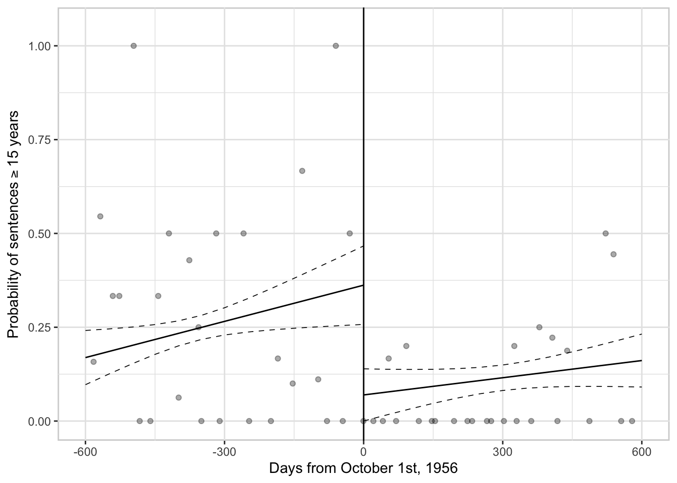
If you plot the regression lines, it would be nice to show that the slopes vary on both sides. If you plot polynomial curves, it would be nice to show that the curves vary on both sides.
RDD Estimation
We run the rdrobust package.
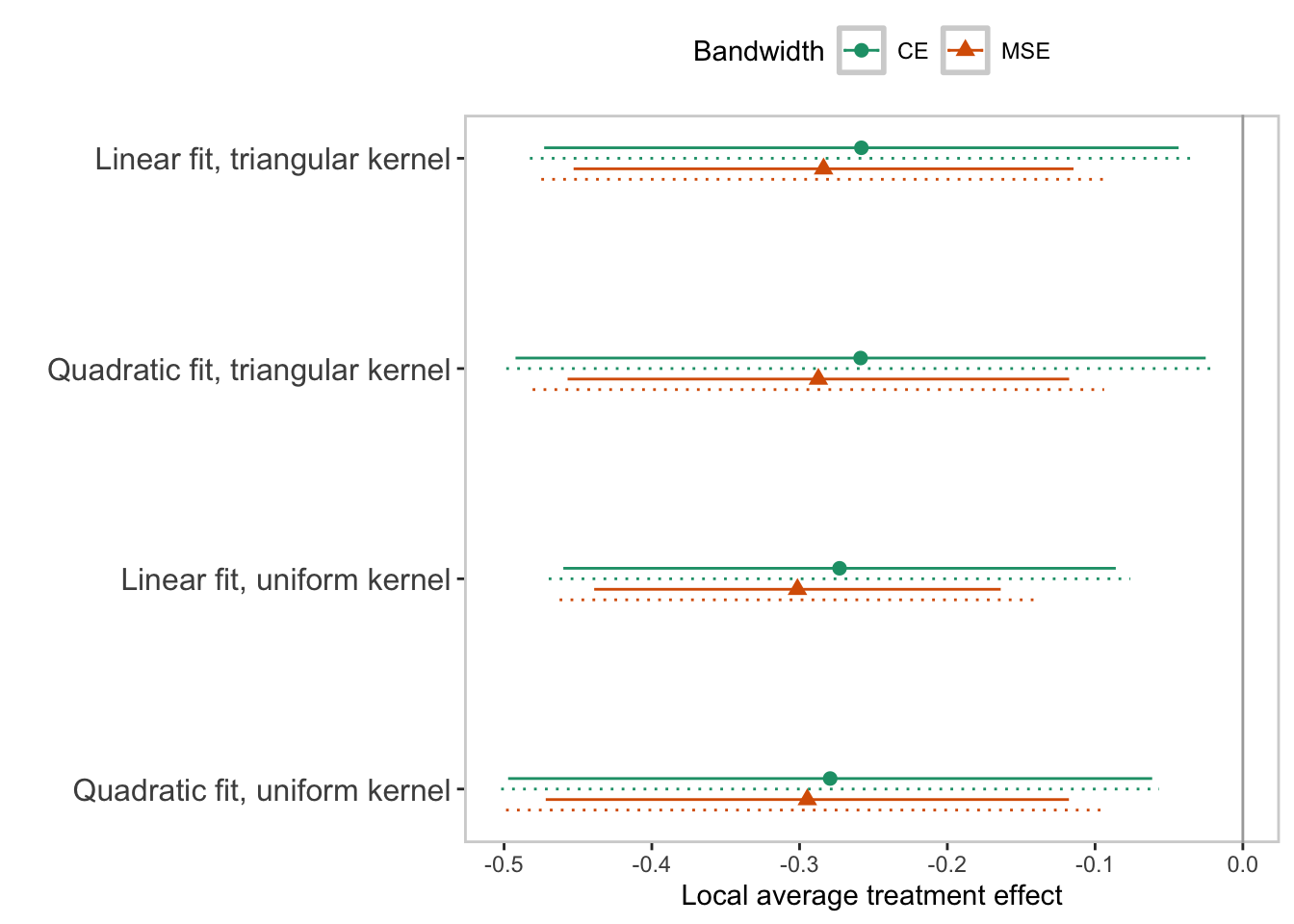
Coefficient plot: various kernal weights and bandwidths
d2h15 <-civilian$d2h15
timediff <-civilian$timediff

#DV, running variable, and covariates of the RD models
Z<-civilian[,c("age","male","islander","d2_per","weapon","subversion",
               "leakmilitary","presreyearr_l")]

m1<-rdrobust(d2h15, timediff, kernel = "tri",bwselect="cerrd", p = 1,
             covs=Z,masspoints = "adjust") #linear fit, triangular kernel, CE bw
m2<-rdrobust(d2h15, timediff, kernel = "tri",bwselect="cerrd", p = 2,
             covs=Z,masspoints = "adjust") #quadratic fit, triangular kernel, CE bw
m3<-rdrobust(d2h15, timediff, kernel = "uni",bwselect="cerrd", p = 1,
             covs=Z,masspoints = "adjust") #linear fit, uniform kernel, CE bw
m4<-rdrobust(d2h15, timediff, kernel = "uni",bwselect="cerrd", p = 2,
             covs=Z,masspoints = "adjust",bwcheck=280) #quadratic fit, uniform kernel, CE bw
m5<-rdrobust(d2h15, timediff, kernel = "tri",bwselect="mserd", p = 1,
             covs=Z,masspoints = "adjust") #linear fit, triangular kernel, MSE bw
m6<-rdrobust(d2h15, timediff, kernel = "tri",bwselect="mserd", p = 2,
             covs=Z,masspoints = "adjust") #quadratic fit, triangular kernel, MSE bw
m7<-rdrobust(d2h15, timediff, kernel = "uni",bwselect="mserd", p = 1,
             covs=Z,masspoints = "adjust") #linear fit, uniform kernel, MSE bw
m8<-rdrobust(d2h15, timediff, kernel = "uni",bwselect="mserd", p = 2,
             covs=Z,masspoints = "adjust") #quadratic fit, uniform kernel, MSE bw

r<-NULL
for(i in 1:8){
  r<-rbind(r,cbind(get(paste0("m", i))$coef[3],get(paste0("m", i))$ci[2,1],get(paste0("m", i))$ci[2,2],
                   get(paste0("m", i))$ci[3,1],get(paste0("m", i))$ci[3,2]))
}
r<-data.frame(r)
colnames(r)<-c("resp","bclower","bcupper","rlower","rupper")
r$trt <-c(3,2,1,0,2.9,1.9,0.9,-0.1)
r$bw<-c("CE","CE","CE","CE","MSE","MSE","MSE","MSE")

#Plot the LATE point estimates and 95% CI
ggplot(r, aes(resp,trt,color=bw))+
  geom_pointrange(aes(xmin = bclower, xmax = bcupper,shape=bw))+
  geom_linerange(aes(y=trt-0.05,xmin = rlower, xmax = rupper),linetype=3)+
  theme(panel.grid.major =element_blank(),
        panel.grid.minor =element_blank(),
        legend.position="top",legend.direction = "horizontal",
        axis.text.y = element_text(size =12),
        strip.text = element_text(size =12),
        panel.background = element_rect(linewidth = 1,colour = "lightgray",fill='white'))+
  scale_y_continuous("",breaks=c(2.95,1.95,0.95,-0.05),
                     labels=c("Linear fit, triangular kernel",
                              "Quadratic fit, triangular kernel",
                              "Linear fit, uniform kernel",
                              "Quadratic fit, uniform kernel"))+
  scale_color_brewer("Bandwidth",palette = "Dark2")+
  scale_shape_discrete("Bandwidth")+
  geom_vline(xintercept = 0, color = "darkgray")+
  scale_x_continuous("Local average treatment effect")
Regression table
d2h15<-civilian$d2h15
timediff<-civilian$timediff

#DV, running variable, and covariates of the RD models
Z<-civilian[,c("age","male","islander","d2_per","weapon","subversion",
               "leakmilitary","presreyearr_l")]

m1<-rdrobust(d2h15, timediff, kernel = "tri",bwselect="cerrd", p = 1,
             covs=Z,masspoints = "adjust") #linear fit, triangular kernel, CE bw

m2<-rdrobust(d2h15, timediff, kernel = "tri",bwselect="cerrd", p = 2,
             covs=Z,masspoints = "adjust") #quadratic fit, triangular kernel, CE bw

m3<-rdrobust(d2h15, timediff, kernel = "uni",bwselect="cerrd", p = 1,
             covs=Z,masspoints = "adjust") #linear fit, uniform kernel, CE bw

m4<-rdrobust(d2h15, timediff, kernel = "uni",bwselect="cerrd", p = 2,
             covs=Z,masspoints = "adjust",bwcheck=280) #quadratic fit, uniform kernel, CE bw

m5<-rdrobust(d2h15, timediff, kernel = "tri",bwselect="mserd", p = 1,
             covs=Z,masspoints = "adjust") #linear fit, triangular kernel, MSE bw

m6<-rdrobust(d2h15, timediff, kernel = "tri",bwselect="mserd", p = 2,
             covs=Z,masspoints = "adjust") #quadratic fit, triangular kernel, MSE bw

m7<-rdrobust(d2h15, timediff, kernel = "uni",bwselect="mserd", p = 1,
             covs=Z,masspoints = "adjust") #linear fit, uniform kernel, MSE bw

m8<-rdrobust(d2h15, timediff, kernel = "uni",bwselect="mserd", p = 2,
             covs=Z,masspoints = "adjust") #quadratic fit, uniform kernel, MSE bw

r<-NULL
for(i in 1:8){
  r<-cbind(r,rbind(round(get(paste0("m", i))$coef[3],3),
                   paste0("[",round(get(paste0("m", i))$ci[2,1],3),", ",round(get(paste0("m", i))$ci[2,2],3),"]"),
                   paste0("[",round(get(paste0("m", i))$ci[3,1],3),", ",round(get(paste0("m", i))$ci[3,2],3),"]"),
                   round(get(paste0("m", i))$bws[1,1]),
                   sum(get(paste0("m", i))$N_h)))
}
r<-data.frame(r)
r
## X1 X2 X3 X4
## 1 -0.258 -0.259 -0.273 -0.279
## 2 [-0.473, -0.043] [-0.492, -0.025] [-0.46, -0.086] [-0.497, -0.061]
## 3 [-0.483, -0.034] [-0.499, -0.019] [-0.47, -0.076] [-0.502, -0.057]
## 4 407 755 440 740
## 5 177 471 205 461
## X5 X6 X7 X8
## 1 -0.284 -0.287 -0.301 -0.295
## 2 [-0.453, -0.115] [-0.457, -0.118] [-0.439, -0.164] [-0.472, -0.118]
## 3 [-0.475, -0.093] [-0.481, -0.094] [-0.462, -0.14] [-0.499, -0.091]
## 4 625 1232 675 945
## 5 322 1144 378 725The table follows the information below:
- LATE
- Bias-corrected 95% CI
- Robust 95% CI
- Bandwidth (days)
- Effective N
- Polynomial order: Linear Quadratic Linear Quadratic Linear Quadratic Linear Quadratic
- Weight: Triangular Triangular Uniform Uniform Triangular Triangular Uniform Uniform
RDD Assumption tests
Covariates continuity/smoothness
Testing for discontinuities in covariates and types of offenses
m1<-rdrobust(civilian$age, civilian$timediff, kernel = "tri",bwselect="cerrd", p = 1,masspoints = "adjust") #age
m2<-rdrobust(civilian$male, civilian$timediff, kernel = "tri",bwselect="cerrd", p = 1,masspoints = "adjust") #male
m3<-rdrobust(civilian$islander, civilian$timediff, kernel = "tri",bwselect="cerrd", p = 1,masspoints = "adjust") #islander
m4<-rdrobust(civilian$d2_per, civilian$timediff, kernel = "tri",bwselect="cerrd", p = 1,masspoints = "adjust") #N of codefendants
m5<-rdrobust(civilian$weapon, civilian$timediff, kernel = "tri",bwselect="cerrd", p = 1,masspoints = "adjust") #weapon
m6<-rdrobust(civilian$subversion, civilian$timediff, kernel = "tri",bwselect="cerrd", p = 1,masspoints = "adjust") #committing subversion
m7<-rdrobust(civilian$leakmilitary, civilian$timediff, kernel = "tri",bwselect="cerrd", p = 1,masspoints = "adjust") #leaking military intelligence
m8<-rdrobust(civilian$presreyearr_l, civilian$timediff, kernel = "tri",bwselect="cerrd", p = 1,masspoints = "adjust") #president review t-1
m9<-rdrobust(civilian$d2_maj, civilian$timediff, kernel = "tri",bwselect="cerrd", p = 1,masspoints = "adjust") #major offenses
m10<-rdrobust(civilian$d2_mid, civilian$timediff, kernel = "tri",bwselect="cerrd", p = 1,masspoints = "adjust") #medium offenses
m11<-rdrobust(civilian$d2_819, civilian$timediff, kernel = "tri",bwselect="cerrd", p = 1,masspoints = "adjust") #minor offenses

r<-NULL
for(i in 1:11){
  r<-rbind(r,cbind(round(get(paste0("m", i))$coef[3],3),
                   paste0("[",round(get(paste0("m", i))$ci[3,1],4)," ,",round(get(paste0("m", i))$ci[3,2],4),"]"),
                   round(get(paste0("m", i))$bws[1,1]),
                   sum(get(paste0("m", i))$N_h)))
}
r<-data.frame(r)
colnames(r)<-c("coefficient","robust CI", "bw","n")
r## coefficient robust CI bw n
## 1 1.29 [-2.3467 ,4.9259] 598 490
## 2 0.033 [-0.0267 ,0.0936] 570 462
## 3 0.13 [-0.1328 ,0.3919] 375 228
## 4 0.181 [-0.0608 ,0.422] 99 79
## 5 0.003 [-0.0012 ,0.0064] 580 474
## 6 0.007 [-0.0674 ,0.0814] 728 671
## 7 0.011 [-0.0238 ,0.0461] 869 841
## 8 -0.002 [-0.0045 ,5e-04] 73 59
## 9 0.097 [-0.1199 ,0.3134] 393 143
## 10 0.042 [-0.2719 ,0.3567] 480 220
## 11 -0.158 [-0.5341 ,0.2178] 402 157## density test ------------------------------------------------------------
summary(rddensity(civilian$timediff))##
## Manipulation testing using local polynomial density estimation.
##
## Number of obs = 9035
## Model = unrestricted
## Kernel = triangular
## BW method = estimated
## VCE method = jackknife
##
## c = 0 Left of c Right of c
## Number of obs 4137 4898
## Eff. Number of obs 294 185
## Order est. (p) 2 2
## Order bias (q) 3 3
## BW est. (h) 582.178 599.12
##
## Method T P > |T|
## Robust 0.3131 0.7542##
## P-values of binomial tests (H0: p=0.5).
##
## Window Length <c >=c P>|T|
## 79.000 + 79.000 20 45 0.0026
## 134.909 + 136.791 36 56 0.0470
## 190.817 + 194.582 55 69 0.2429
## 246.726 + 252.373 61 80 0.1293
## 302.635 + 310.164 71 92 0.1170
## 358.544 + 367.955 98 107 0.5764
## 414.452 + 425.746 161 125 0.0383
## 470.361 + 483.537 197 151 0.0157
## 526.270 + 541.329 213 180 0.1064
## 582.178 + 599.120 294 185 0.0000Donut hole test
Table A.8. Regression discontinuity of the 1956 reform on sentence severity for civilian dissidents (donut-hole test)
# 1 month donut-hole
d2h15<-civilian$d2h15[abs(civilian$timediff) >= 31]
timediff<-civilian$timediff[abs(civilian$timediff) >= 31]
Z<-civilian[abs(civilian$timediff) >= 31,
            c("age","male","islander","d2_per","weapon","subversion",
              "leakmilitary","presreyearr_l")]
m1<-rdrobust(d2h15,timediff,kernel = "tri",p = 1,covs=Z,bwselect="cerrd", bwcheck=250,masspoints = "adjust")

# 3 months donut-hole
d2h15<-civilian$d2h15[abs(civilian$timediff) >= 91]
timediff<-civilian$timediff[abs(civilian$timediff) >= 91]
Z<-civilian[abs(civilian$timediff) >=91,
            c("age","male","islander","d2_per","weapon","subversion",
              "leakmilitary","presreyearr_l")]
m2<-rdrobust(d2h15,timediff, kernel = "tri",p = 1, covs=Z,bwselect="cerrd", bwcheck=250,masspoints = "adjust")


r<-NULL
for(i in 1:2){
  r<-rbind(r,cbind(round(get(paste0("m",i))$coef[1],3),
                   paste0("[",round(get(paste0("m",i))$ci[3,1],3),",",round(get(paste0("m",i))$ci[3,2],3),"]"),
                   round(get(paste0("m",i))$bws[1,1]),
                   sum(get(paste0("m",i))$N_h)))
           }
r<-data.frame(r)
r## X1 X2 X3 X4
## 1 -0.257 [-0.487,-0.069] 525 256
## 2 -0.417 [-0.745,-0.173] 509 222The result remains the same when carving out 1 months or 3 months of observations near the cutoff, supporting the non-sorting/manipulation assumption.
Autoregression test
Table A.9. Regression discontinuity of the 1956 reform on sentence severity for civilian dissidents (with lagged dependent variable)
d2h15<-civilian$d2h15
timediff<-civilian$timediff

#include monthly average of the dependent variable in t − 1 as a covariate
Z<-civilian[,c("age","male","islander","d2_per","weapon","subversion",
               "leakmilitary","presreyearr_l","d2h15_lm")]


m1<-rdrobust(d2h15, timediff, kernel = "tri",bwselect="cerrd", p = 1,
             covs=Z,masspoints = "adjust") #linear fit, triangular kernel, CE bw
m2<-rdrobust(d2h15, timediff, kernel = "tri",bwselect="cerrd", p = 2,
             covs=Z,masspoints = "adjust") #quadratic fit, triangular kernel, CE bw
m3<-rdrobust(d2h15, timediff, kernel = "uni",bwselect="cerrd", p = 1,
             covs=Z,masspoints = "adjust") #linear fit, uniform kernel, CE bw
m4<-rdrobust(d2h15, timediff, kernel = "uni",bwselect="cerrd", p = 2,
             covs=Z,masspoints = "adjust",bwcheck=250) #quadratic fit, uniform kernel, CE bw
m5<-rdrobust(d2h15, timediff, kernel = "tri",bwselect="mserd", p = 1,
             covs=Z,masspoints = "adjust") #linear fit, triangular kernel, MSE bw
m6<-rdrobust(d2h15, timediff, kernel = "tri",bwselect="mserd", p = 2,
             covs=Z,masspoints = "adjust") #quadratic fit, triangular kernel, MSE bw
m7<-rdrobust(d2h15, timediff, kernel = "uni",bwselect="mserd", p = 1,
             covs=Z,masspoints = "adjust") #linear fit, uniform kernel, MSE bw
m8<-rdrobust(d2h15, timediff, kernel = "uni",bwselect="mserd", p = 2,
             covs=Z,masspoints = "adjust") #quadratic fit, uniform kernel, MSE bw

r<-NULL
for(i in 1:8){
  r<-cbind(r,rbind(round(get(paste0("m", i))$coef[3],3),
                   paste0("[",round(get(paste0("m", i))$ci[2,1],3),", ",round(get(paste0("m", i))$ci[2,2],3),"]"),
                   paste0("[",round(get(paste0("m", i))$ci[3,1],3),", ",round(get(paste0("m", i))$ci[3,2],3),"]"),
                   round(get(paste0("m", i))$bws[1,1]),
                   sum(get(paste0("m", i))$N_h)))
}
r<-data.frame(r)
r
## X1 X2 X3 X4
## 1 -0.25 -0.258 -0.228 -0.294
## 2 [-0.461, -0.038] [-0.494, -0.022] [-0.433, -0.022] [-0.524, -0.065]
## 3 [-0.472, -0.028] [-0.501, -0.016] [-0.442, -0.013] [-0.529, -0.06]
## 4 419 753 393 697
## 5 175 447 149 395
## X5 X6 X7 X8
## 1 -0.281 -0.294 -0.321 -0.281
## 2 [-0.457, -0.105] [-0.474, -0.115] [-0.485, -0.157] [-0.467, -0.095]
## 3 [-0.479, -0.083] [-0.498, -0.091] [-0.506, -0.136] [-0.496, -0.066]
## 4 642 1227 602 958
## 5 314 1110 291 712Manipulation assumption test
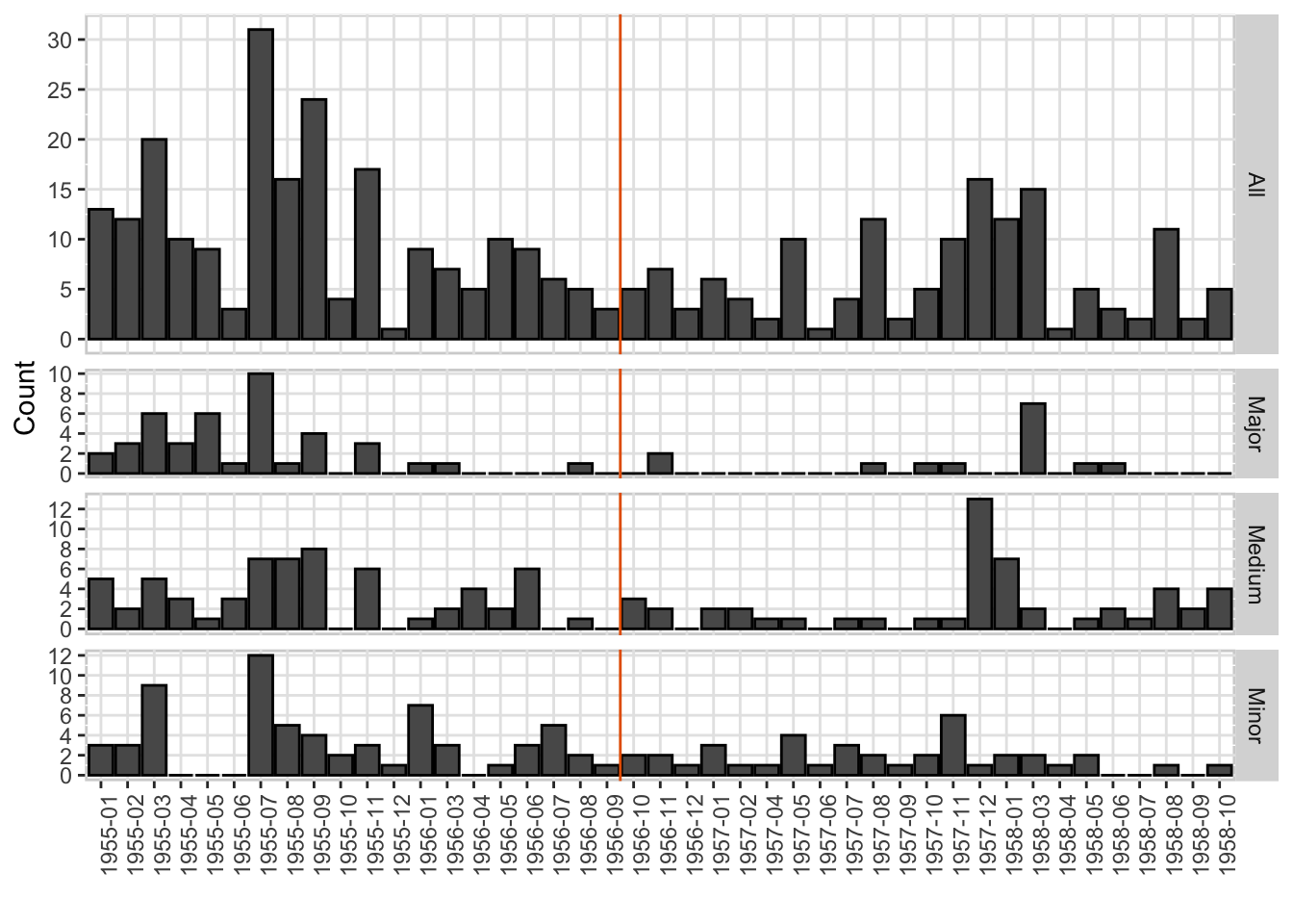
The goal is to show that observations remain stable before and after the cutoff–no obvious manipulation happens.
Figure A.1. Frequency of civilian dissident cases around Oct. 1st, 1956.
freq<-civilian[!is.na(civilian$d2h15),]
freq<-freq[!is.na(freq$minyy),]

case<-freq %>%
  group_by(minyy,minym) %>%
  summarize(d2_all = n(),
            d2_maj=sum(d2_maj,na.rm=T),d2_mid=sum(d2_mid,na.rm=T),d2_min=sum(d2_819,na.rm=T))
#aggregate data to monthly frequencies, divided by types of offenses

case<-as.data.frame(case)
r<-names(table(case$minym))
case$minym<-factor(case$minym, levels=r)
long<-reshape(data=case,idvar="minym",varying=names(case[,3:6]),
              timevar="type",direction="long",sep="_")
long$type<-factor(long$type, labels=c("All","Major", "Medium","Minor"))

ggplot(long[case$minyy>=1955&case$minyy<=1958&!case$minym%in%c("1958-11","1958-12"),],
       aes(minym,d2))+geom_col(col="black")+facet_grid(rows = vars(type),scales = "free", space = "free")+
  theme( panel.grid.major =  element_line(colour = "grey90"), panel.background = element_rect(size = 1,colour = "lightgray",fill='white'),
         axis.text.x = element_text(angle = 90, vjust = 1, hjust=1.5))+
  scale_x_discrete("")+scale_y_continuous("Count",breaks = breaks_extended(8))+
  geom_vline(xintercept = 20.5, color = "#E66100")