Panel Data Design
Goal of today
We learn how to estimate models with random effects and fixed effects.
The source code for this lab can be found here.
The data used for this lab can be found here.
Preparation
Load packages
library(plm)
# install.packages("plm", dependencies = TRUE)
If you receive error messages, saying “Error in library(plm) : there is no package called ‘plm’” then delete the pound sign in the following line and execute it. Otherwise, move on.
rm(list = ls())       # delete everything in the memory
library(foreign)      # for read.dta
library(ggplot2)      # for graphics
library(stargazer)    # Regression table
##
## Please cite as:## Hlavac, Marek (2022). stargazer: Well-Formatted Regression and Summary Statistics Tables.## R package version 5.2.3. https://CRAN.R-project.org/package=stargazerlibrary(effects) # for effect## Loading required package: carData## lattice theme set by effectsTheme()
## See ?effectsTheme for details.library(plm) # for plm
# remotes::install_github("jhelvy/renderthis")
# remotes::install_github('rstudio/chromote')Age and life satisfaction
Load the beatles data.
bt <- read.dta("beatles.dta")
# Take a look:
bt
## year id name age lsat
## 1 1968 1 John 28 8
## 2 1969 1 John 29 6
## 3 1970 1 John 30 5
## 4 1968 2 Paul 26 5
## 5 1969 2 Paul 27 2
## 6 1970 2 Paul 28 1
## 7 1968 3 George 25 4
## 8 1969 3 George 26 3
## 9 1970 3 George 27 1
## 10 1968 4 Ringo 28 9
## 11 1969 4 Ringo 29 8
## 12 1970 4 Ringo 30 6In a hypothetical survey, we asked four people (John, Paul, George, and Ringo) to rate how satisfied they are on a scale from 0 to 10. We conducted this survey three times (1968, 1969, and 1970). The variable lsat records the respondents’ answers in each year. This is our DV. Other variables should be self-explanatory.
Scatterplot ignoring the panel structure
g <- ggplot(bt, aes(x = age, y = lsat)) + geom_point()
g <- g + xlab("Age") + ylab("Life satisfaction") + theme_bw()
g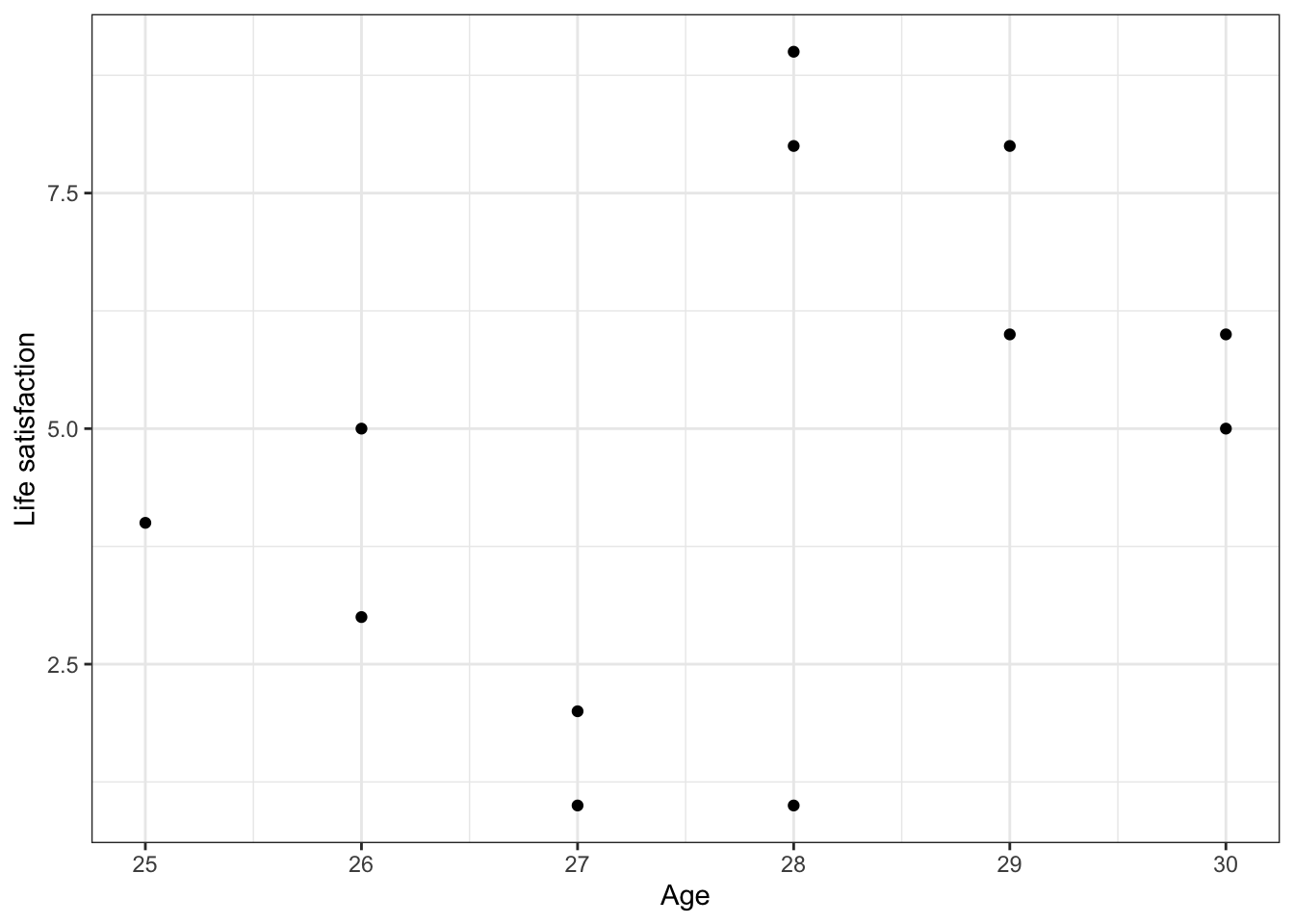
It “appears” that there is a positive relationship between age and life satisfaction, implying that, as you get older, you tend to be more satisfied with life (to put it more accurately, you say you are more satisfied with life).
Now to add a regression line to the scatter plot, we use the geom_smooth function, as follows.
g <- g + geom_smooth(method = lm, alpha = 0)
g
## `geom_smooth()` using formula = 'y ~ x'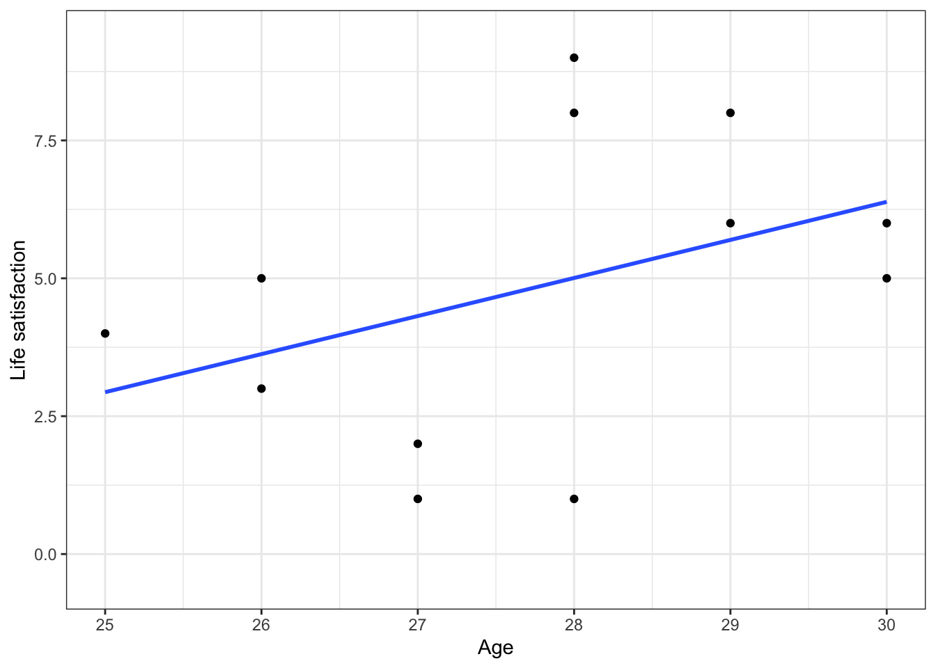
“method = lm” means that we ask R to fit a line, not a curve. “alpha = 0” means that we ask R to make the confidence bands to be completely transparent. You can tweak them to see what happens.
g <- g + geom_smooth(method = lm, alpha = 0.5)
g
## `geom_smooth()` using formula = 'y ~ x'
## `geom_smooth()` using formula = 'y ~ x'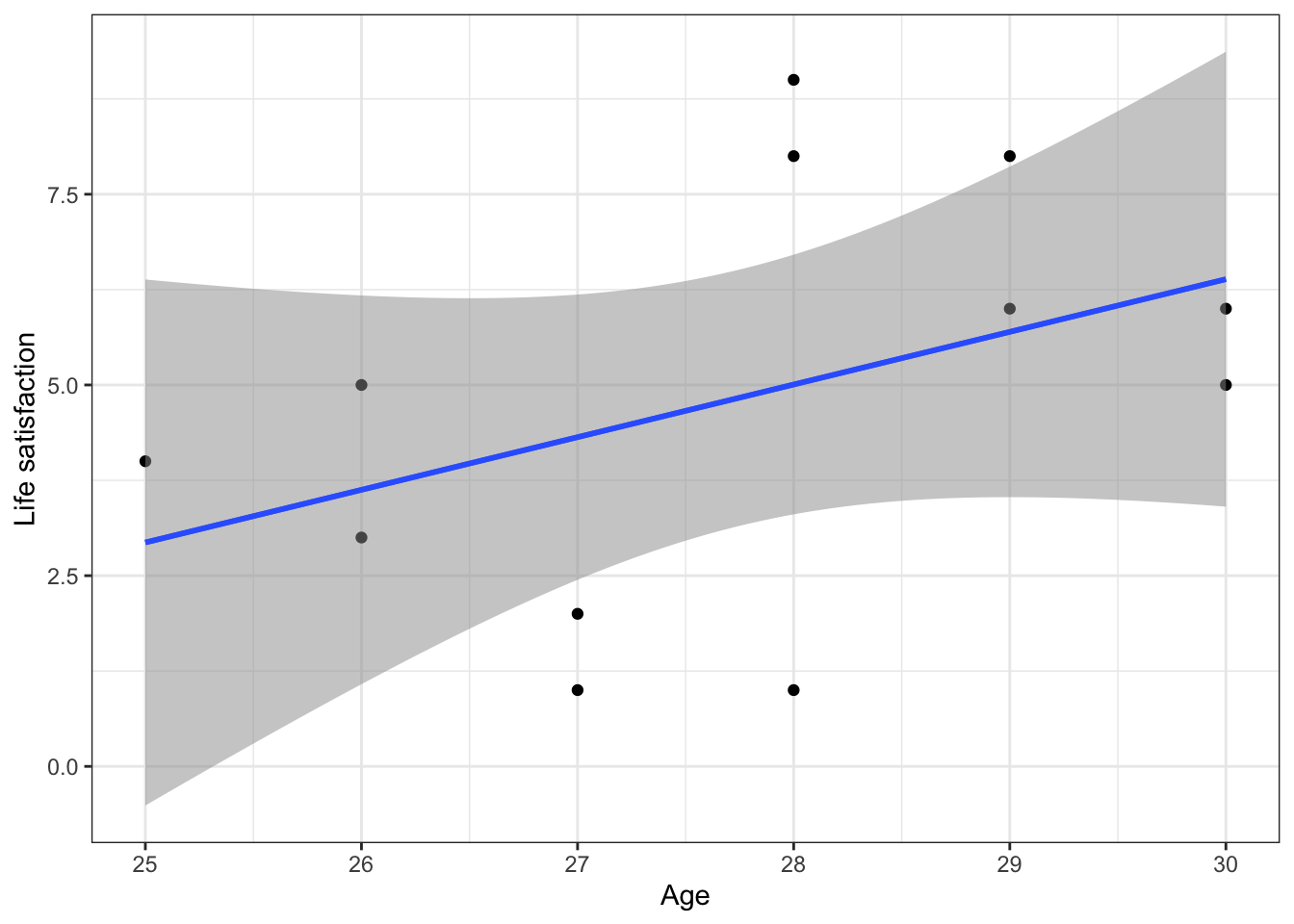
As we saw in the lecture, this apparent positive effect of age is just an artifact caused by ignoring the panel structure.
In order to create a scatterplot where data points for different people are given different colors, we modify the aes argument as follows.
g <- ggplot(bt, aes(x = age, y = lsat, colour = name)) + geom_point()
g <- g + xlab("Age") + ylab("Life satisfaction") + theme_bw()
g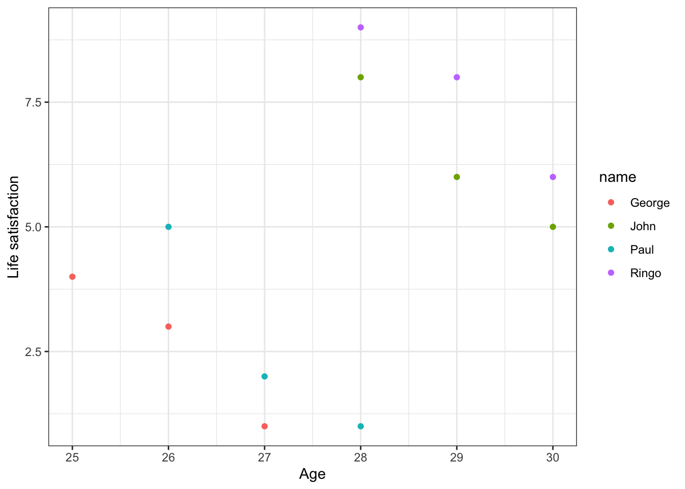
# "colour = name" (NB: British spelling) means that we ask R to use different colors depending on the value of the "name" variable.We have also learned before how to insert texts into a graph.
g <- ggplot(bt, aes(x = age, y = lsat, colour=name)) + geom_point()
g <- g + geom_text(aes(y = lsat-.5, label = name)) + theme_bw()
g <- g + ylab("Age") + xlab("Life satisfaction")
g <- g + theme(legend.position = "none")
g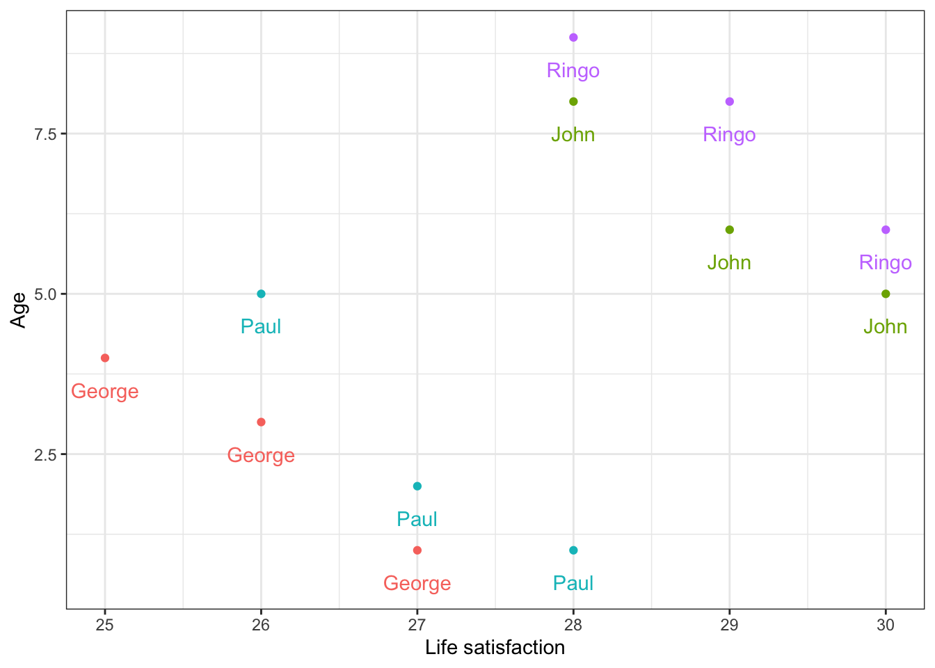
We can clearly see that age actually has a negative, not positive, effect on lsat if we make a within-unit (over time) comparison.
Panel data regression: The plm package
The first step in using the plm package is to declare that the data set you have is a panel data set. We do this by using the plm.data function.
As we learned in the lecture, we supply the information about the cross-sectional unit and the time unit using the index argument.
bt.panel <- pdata.frame(bt, index = c("name", "year") )Now we are ready to estimate models for panel data.
Model 1: Pooled model
fit.bt.pool <- plm(lsat ~ age, data = bt.panel, model = "pooling")

stargazer(fit.bt.pool, type = "text")
##
## ========================================
## Dependent variable:
## ---------------------------
## lsat
## ----------------------------------------
## age 0.690
## (0.491)
##
## Constant -14.322
## (13.656)
##
## ----------------------------------------
## Observations 12
## R2 0.165
## Adjusted R2 0.081
## F Statistic 1.973 (df = 1; 10)
## ========================================
## Note: *p<0.1; **p<0.05; ***p<0.01As we learned in the lecture, the results should be identical to a simple linear regression results we’d obtain using the familiar lm function.
fit.bt.slr <- lm(lsat ~ age, data = bt)

stargazer(fit.bt.pool, fit.bt.slr, type = "text")
##
## =====================================================
## Dependent variable:
## ----------------------------
## lsat
## panel OLS
## linear
## (1) (2)
## -----------------------------------------------------
## age 0.690 0.690
## (0.491) (0.491)
##
## Constant -14.322 -14.322
## (13.656) (13.656)
##
## -----------------------------------------------------
## Observations 12 12
## R2 0.165 0.165
## Adjusted R2 0.081 0.081
## Residual Std. Error 2.612 (df = 10)
## F Statistic (df = 1; 10) 1.973 1.973
## =====================================================
## Note: *p<0.1; **p<0.05; ***p<0.01Model 2: FE model
To estimate a fixed-effects (FE) model, a.k.a., a within-effect model, we replace “pooling” with “within”, as follows.
fit.bt.fe <- plm(lsat ~ age, data = bt.panel, model = "within")

stargazer(fit.bt.pool, fit.bt.fe, type = "text")
##
## =====================================================
## Dependent variable:
## ----------------------------------------
## lsat
## (1) (2)
## -----------------------------------------------------
## age 0.690 -1.625***
## (0.491) (0.166)
##
## Constant -14.322
## (13.656)
##
## -----------------------------------------------------
## Observations 12 12
## R2 0.165 0.932
## Adjusted R2 0.081 0.893
## F Statistic 1.973 (df = 1; 10) 95.919*** (df = 1; 7)
## =====================================================
## Note: *p<0.1; **p<0.05; ***p<0.01The estimated coefficient for age is now negative and significant, as we would expect from the revised scatterplot.
We could obtain the same estimate for the effect of age (-1.625) by including individual-specific intercepts manually (adding fixed effects dummies).
bt $ John <- ifelse(bt $ name == "John", 1, 0) # create dummies to account for the grouping structure in the data, when we examine lsat ~ age
bt $ Paul <- ifelse(bt $ name == "Paul", 1, 0)
bt $ George <- ifelse(bt $ name == "George", 1, 0)
bt $ Ringo <- ifelse(bt $ name == "Ringo", 1, 0)

# model with four dummies (no intercept)
fit.bt.fe.2 <- lm(lsat ~ age + John + Paul + Ringo + George + 0,
  data = bt)

# model with three dummies (with intercept)
fit.bt.fe.3 <- lm(lsat ~ age + John + Paul +  Ringo + George ,
  data = bt)

stargazer(fit.bt.fe, fit.bt.fe.2, fit.bt.fe.3, type = "text")
##
## ===============================================================================================
## Dependent variable:
## ------------------------------------------------------------------
## lsat
## panel OLS
## linear
## (1) (2) (3)
## -----------------------------------------------------------------------------------------------
## age -1.625*** -1.625*** -1.625***
## (0.166) (0.166) (0.166)
##
## John 53.458*** 8.542***
## (4.819) (0.628)
##
## Paul 46.542*** 1.625***
## (4.488) (0.418)
##
## Ringo 54.792*** 9.875***
## (4.819) (0.628)
##
## George 44.917***
## (4.322)
##
## Constant 44.917***
## (4.322)
##
## -----------------------------------------------------------------------------------------------
## Observations 12 12 12
## R2 0.932 0.996 0.981
## Adjusted R2 0.893 0.993 0.970
## Residual Std. Error (df = 7) 0.469 0.469
## F Statistic 95.919*** (df = 1; 7) 327.335*** (df = 5; 7) 90.953*** (df = 4; 7)
## ===============================================================================================
## Note: *p<0.1; **p<0.05; ***p<0.01stargazer(fit.bt.fe, fit.bt.fe.2, fit.bt.fe.3, type = "text", omit.stat = c("f"))##
## ==========================================================
## Dependent variable:
## -----------------------------
## lsat
## panel OLS
## linear
## (1) (2) (3)
## ----------------------------------------------------------
## age -1.625*** -1.625*** -1.625***
## (0.166) (0.166) (0.166)
##
## John 53.458*** 8.542***
## (4.819) (0.628)
##
## Paul 46.542*** 1.625***
## (4.488) (0.418)
##
## Ringo 54.792*** 9.875***
## (4.819) (0.628)
##
## George 44.917***
## (4.322)
##
## Constant 44.917***
## (4.322)
##
## ----------------------------------------------------------
## Observations 12 12 12
## R2 0.932 0.996 0.981
## Adjusted R2 0.893 0.993 0.970
## Residual Std. Error (df = 7) 0.469 0.469
## ==========================================================
## Note: *p<0.1; **p<0.05; ***p<0.01These three results are just three different ways of representing a single model.
(Adjusted R^2 is different because plm uses a slightly different method in penalizing models with additional variables.)
The fixest package
These days, feols function from the fixest package becomes more popular
library(fixest)

fit.bt.fe.4 <- feols(lsat ~ age | name, data = bt.panel, panel.id = ~ name)
You can do both FE and clustered standard errors together, making it more robust.
Unfortunately, stargazer hasn’t incorporated this package so we need to use other packages to export our results.
library(texreg)

screenreg(list(fit.bt.fe.4),
          caption = "FE-OLS models with clustered standard errors at individual level.",
       label = "tab:ols",
       digits = 4,
       caption.above = T,
       include.nobs = TRUE,
       include.ci = TRUE,
       include.rsquared = TRUE,
       include.adjrs = TRUE,
       include.rmse = TRUE)
##
## =================================
## Model 1
## ---------------------------------
## age -1.6250 **
## (0.1311)
## ---------------------------------
## Num. obs. 12
## Num. groups: name 4
## R^2 (full model) 0.9811
## R^2 (proj model) 0.9320
## Adj. R^2 (full model) 0.9703
## Adj. R^2 (proj model) 0.9223
## =================================
## *** p < 0.001; ** p < 0.01; * p < 0.05Result is the same with a slightly smaller se.
Model 3: RE model
To estimate a random-effects (RE) model, we simply replace “within” with “random”, as follows.
fit.bt.re <- plm(lsat ~ age, data = bt.panel, model = "random")

stargazer(fit.bt.pool, fit.bt.fe, fit.bt.re, type = "text")
##
## ===============================================================
## Dependent variable:
## --------------------------------------------------
## lsat
## (1) (2) (3)
## ---------------------------------------------------------------
## age 0.690 -1.625*** -1.172***
## (0.491) (0.166) (0.383)
##
## Constant -14.322 37.364***
## (13.656) (10.724)
##
## ---------------------------------------------------------------
## Observations 12 12 12
## R2 0.165 0.932 0.483
## Adjusted R2 0.081 0.893 0.431
## F Statistic 1.973 (df = 1; 10) 95.919*** (df = 1; 7) 9.346***
## ===============================================================
## Note: *p<0.1; **p<0.05; ***p<0.01Tests
To test if FE is necessary or pooled model is enough, we perform an F test
pFtest(fit.bt.fe, fit.bt.pool)##
## F test for individual effects
##
## data: lsat ~ age
## F = 100.9, df1 = 3, df2 = 7, p-value = 4.006e-06
## alternative hypothesis: significant effectsThe p-value is very small, suggesting that FE is much better than the pooled model in terms of model fit.
To test if FE is necessary or RE is enough, we perform a “Hausman test” to compare FE and RE models.
phtest(fit.bt.fe, fit.bt.re)##
## Hausman Test
##
## data: lsat ~ age
## chisq = 1.7151, df = 1, p-value = 0.1903
## alternative hypothesis: one model is inconsistentThe p-value is greater than the conventional threshold, so we fail to reject the null hypothesis that FE and RE models are equivalent (and they are both much better than the pooled model). This means that we can use the random-effects model (which is more efficient), not the fixed-effects model (which is more flexible but less efficient) or the pooled model.
Efficiency: The RE model is typically more efficient (i.e., has smaller standard errors) when the individual-specific effects are uncorrelated with the independent variables.
Flexibility: The FE model is more flexible as it does not assume uncorrelated effects, but it is usually less efficient because it uses up more degrees of freedom by estimating effects for each cross-sectional unit.
Of course, looking at the regression table, the RE model also confirms the relationship we uncovered with the FE model: the effect of age on lsat is negative and significant.