Ordered Logit regression
1. Preparation
rm(list = ls())       # delete everything in the memory
library(foreign)      # for read.dta
library(ggplot2)      # for graphics
library(stargazer) # Regression table##
## Please cite as:## Hlavac, Marek (2022). stargazer: Well-Formatted Regression and Summary Statistics Tables.## R package version 5.2.3. https://CRAN.R-project.org/package=stargazerlibrary(effects) # for effect## Loading required package: carData## lattice theme set by effectsTheme()
## See ?effectsTheme for details.library(MASS) # for plor2. Load the data
Load the Terris & Maoz data set
tm <- read.dta("terrismaoz05.dta")Preemptively drop those observations that have missing values on DV or IVs.
tm <- na.omit(tm[c("medintrus","cumversatil","minreg302","caprat","ally1","lagprmed")])3. Let’s examine the dependent variable
# DV
table(tm$medintrus)##
## None Information/Procedural Directive
## 1244 61 77medintrus is the dependent variable that measures the incidence and intrusiveness of mediation.
It has three ordered categorical values. It appears that the categories are ordered and that R recognizes them as such. We can see that R recognizes this because the category “None” is shown first in the data. If the categories were not recognized by R, the category “Directive” would come first because the letter D comes before the letter N or I.
So we don’t have to do anything about this.
If, the categories were indeed messed up, we can correct it by using the factor function with the ordered, levels, and labels options.
4. Estimate an ordered logit model
fit <- polr(medintrus ~ minreg302 + caprat + ally1 +
              lagprmed + cumversatil,
data = tm, Hess=TRUE) # We also specify Hess=TRUE to have the model return the observed information matrix from optimization (called the Hessian) which is used to get standard errors.## Warning: glm.fit: fitted probabilities numerically 0 or 1 occurredIt gives a Warning message. R is telling us that the predicted probabilities are very close to 0 or 1 for some observations. This might raise some concerns under some circumstances, but we can just ignore this for now.
5. Table of results
stargazer(fit, type = "text")##
## =========================================
## Dependent variable:
## ---------------------------
## medintrus
## -----------------------------------------
## minreg302 0.007**
## (0.003)
##
## caprat -0.008*
## (0.005)
##
## ally1Alliance 1.066***
## (0.211)
##
## lagprmed 0.263***
## (0.060)
##
## cumversatil 0.004***
## (0.0004)
##
## -----------------------------------------
## Observations 1,382
## =========================================
## Note: *p<0.1; **p<0.05; ***p<0.01If you want to use proper variable names, we can supply them using the covariate.labels option.
stargazer(fit, type = "text",
          covariate.labels = c("Minimum Regime Score", "Capability Ratio",
                               "Alliance", "Prior Mediation",
"Conflict Versatility"))##
## ================================================
## Dependent variable:
## ---------------------------
## medintrus
## ------------------------------------------------
## Minimum Regime Score 0.007**
## (0.003)
##
## Capability Ratio -0.008*
## (0.005)
##
## Alliance 1.066***
## (0.211)
##
## Prior Mediation 0.263***
## (0.060)
##
## Conflict Versatility 0.004***
## (0.0004)
##
## ------------------------------------------------
## Observations 1,382
## ================================================
## Note: *p<0.1; **p<0.05; ***p<0.01If you want to save the table in a file, use the “out” option.
## text file
stargazer(fit, type = "text", out = "table.txt",
          covariate.labels = c("Minimum Regime Score", "Capability Ratio",
                               "Alliance", "Prior Mediation",
"Conflict Versatility"))##
## ================================================
## Dependent variable:
## ---------------------------
## medintrus
## ------------------------------------------------
## Minimum Regime Score 0.007**
## (0.003)
##
## Capability Ratio -0.008*
## (0.005)
##
## Alliance 1.066***
## (0.211)
##
## Prior Mediation 0.263***
## (0.060)
##
## Conflict Versatility 0.004***
## (0.0004)
##
## ------------------------------------------------
## Observations 1,382
## ================================================
## Note: *p<0.1; **p<0.05; ***p<0.01# ## html file (to be opened with an internet browser, such as Chrome)
# stargazer(fit, type = "html", out = "table.html",
# covariate.labels = c("Minimum Regime Score", "Capability Ratio",
# "Alliance", "Prior Mediation",
# "Conflict Versatility"))6. Find the cut-point estimates
summary(fit)## Call:
## polr(formula = medintrus ~ minreg302 + caprat + ally1 + lagprmed +
## cumversatil, data = tm, Hess = TRUE)
##
## Coefficients:
## Value Std. Error t value
## minreg302 0.007349 0.0033108 2.220
## caprat -0.008497 0.0046111 -1.843
## ally1Alliance 1.065726 0.2105638 5.061
## lagprmed 0.263148 0.0596778 4.409
## cumversatil 0.003942 0.0003839 10.268
##
## Intercepts:
## Value Std. Error t value
## None|Information/Procedural 4.3434 0.3199 13.5767
## Information/Procedural|Directive 5.0789 0.3352 15.1513
##
## Residual Deviance: 898.8218
## AIC: 912.8218We can see that the first cutpoint is 4.3434 and the second cutpoint is 5.0789.
7. Effect of conflict versatility
Calculate the marginal effects of cumversatil
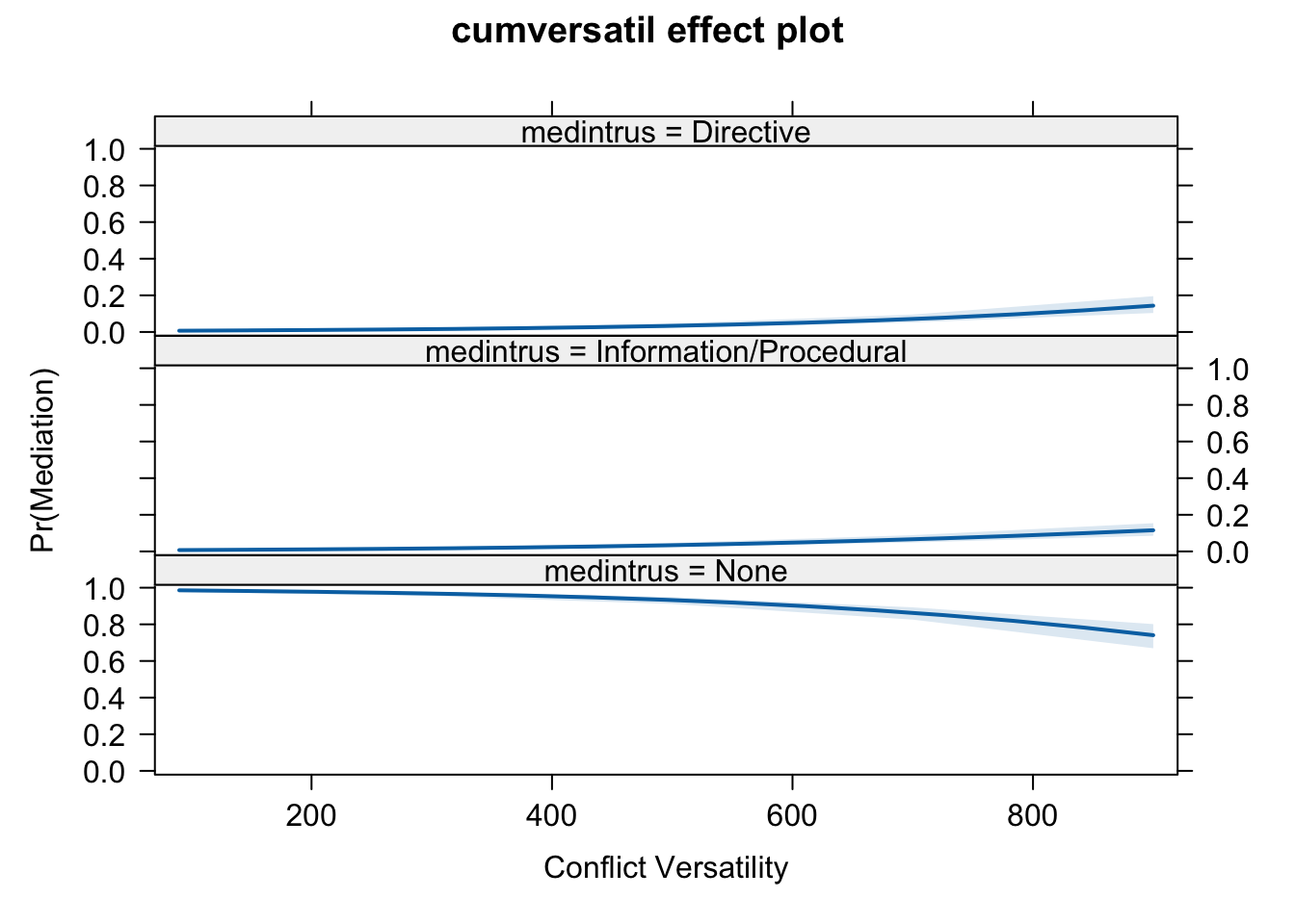
eff.cv <- effect(term = "cumversatil", mod = fit)

eff.cv##
## cumversatil effect (probability) for None
## cumversatil
## 90 300 500 700 900
## 0.9858355 0.9681693 0.9325552 0.8627428 0.7407561
##
## cumversatil effect (probability) for Information/Procedural
## cumversatil
## 90 300 500 700 900
## 0.007325136 0.016317418 0.033942605 0.066407423 0.115600214
##
## cumversatil effect (probability) for Directive
## cumversatil
## 90 300 500 700 900
## 0.006839342 0.015513264 0.033502229 0.070849751 0.143643654Plot the effects
plot(eff.cv, rescale.axis = FALSE,
     xlab = "Conflict Versatility",
     ylab = "Pr(Mediation)", rug = FALSE)
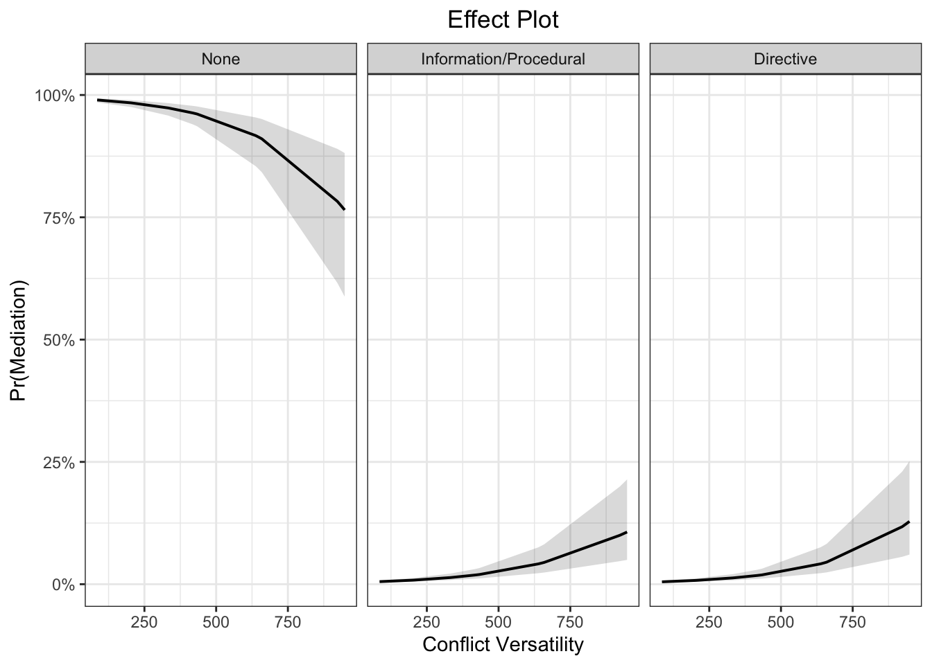
It looks ugly. Let’s do it in ggplot.
library(sjPlot)## #refugeeswelcomeplot_model(fit, type = "pred", terms = c("cumversatil [all]"), ci.lvl = 0.95, bpe.style = "line", robust = T, legend.title = "", vcov.type = c("HC3"), colors="bw") +
theme_bw() +
ggtitle(element_blank()) +
xlab("Conflict Versatility") + ylab("Pr(Mediation)") +
labs(title = "Effect Plot") +
theme(plot.title = element_text(hjust = 0.5)) 
You can save a pdf file by doing this:
# Print the plot to a pdf file
g <-  plot_model(fit, type = "pred", terms = c("cumversatil [all]"), ci.lvl = 0.95, bpe.style = "line", robust = T, legend.title = "", vcov.type = c("HC3"), colors="bw") +
  theme_bw() +
  ggtitle(element_blank()) +
  xlab("Conflict Versatility") + ylab("Pr(Mediation)") +
  labs(title = "Effect Plot") +
  theme(plot.title = element_text(hjust = 0.5))

# ggsave(g, filename = "eff_plot.pdf",width = 8, height = 6, dpi = 200, device = "pdf")
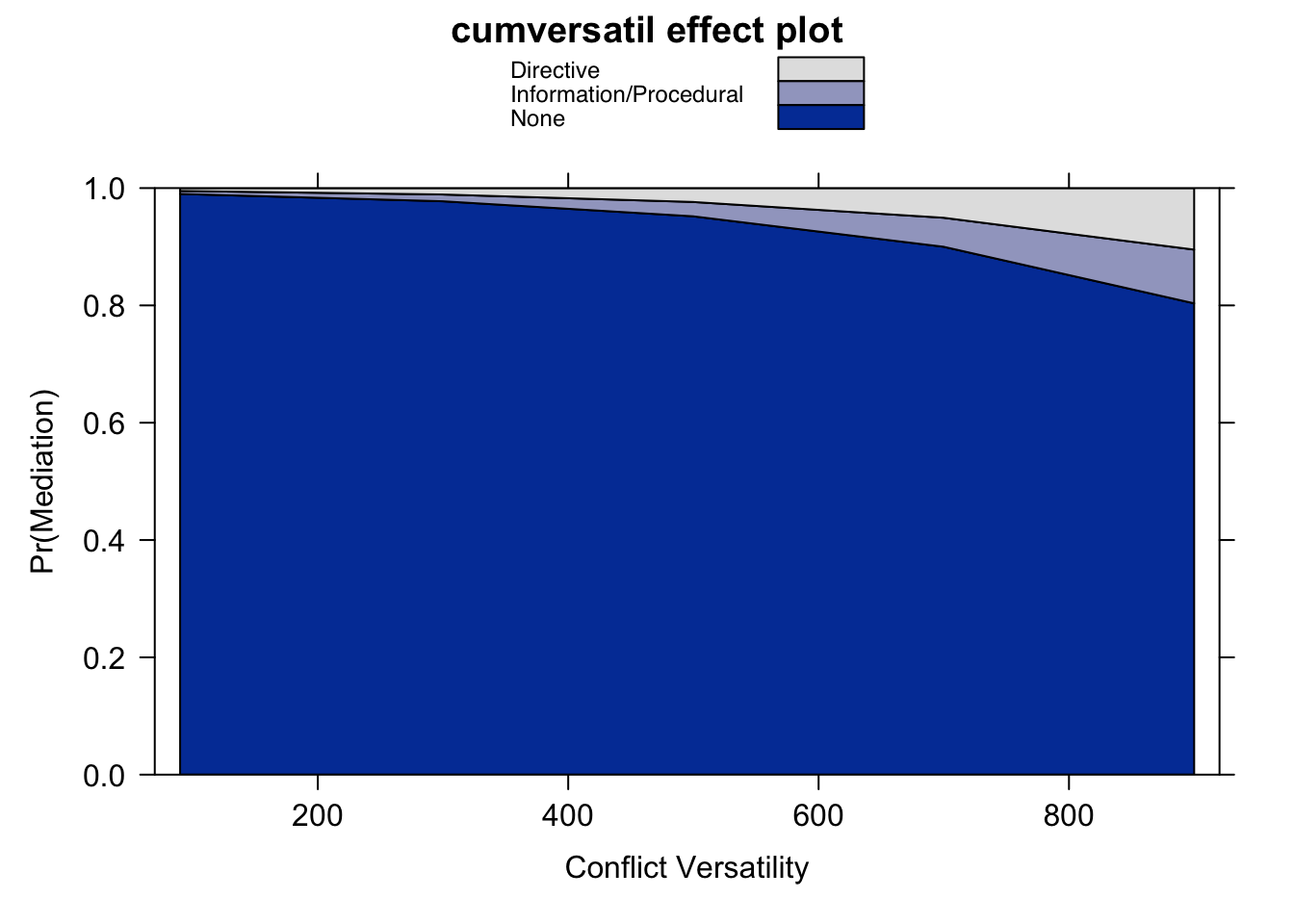
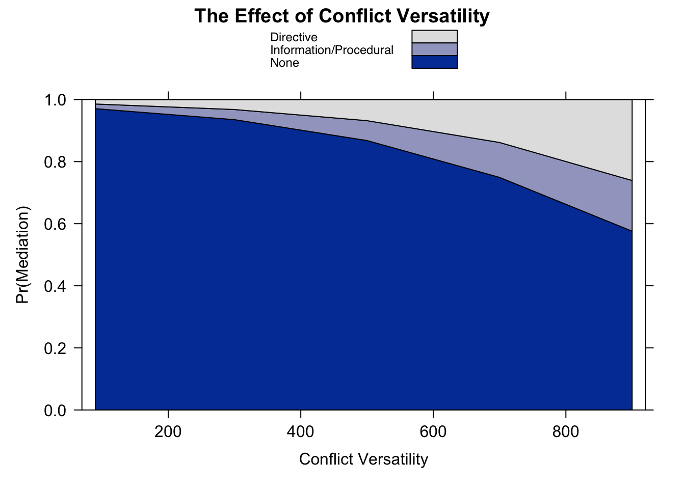
You could also do the area plots if you want. But a big downside is that there is no indication of uncertainty. So I won’t recommend it.
eff.cv.mr.max <- effect(term = "cumversatil", mod = fit, given.values = c("minreg302" = 60))
eff.cv.mr.min <- effect(term = "cumversatil", mod = fit, given.values = c("minreg302" = -90))

# Produce the plot for minimum
plot(eff.cv.mr.min, rescale.axis = FALSE,
     xlab = "Conflict Versatility", ylab = "Pr(Mediation)",
     rug = FALSE, style = "stacked")
# Produce the plot for maximum
plot(eff.cv.mr.max, rescale.axis = FALSE,
     main = "The Effect of Conflict Versatility",
     xlab = "Conflict Versatility", ylab = "Pr(Mediation)",
     rug = FALSE, style = "stacked")