Matching
- Goal Today
- MatchIt: motivation
- PanelMatch: Motivation
- Load replicated data
- Codebook
- Pre-analysis: Visualizing the Treatment Variation Plot
- Decide leads and lags values
- Store the covariates formula
- Construct the Matched Sets
- Plot Freq distribution of the number of matched control units
- Refine matched sets: Compare different matching methods
- DiD Estimation
- Authoritarian reversal and Economic Growth
- Load replicated data
Goal Today
- Learn basic commands in popular packages that estimate causal effects under the various matching framework
- Replicate a few examples in the book for cross-n matching (using
matchIt) - Learn how to do panel data matching (using
PanelMatch)
MatchIt: motivation
Matching has been heavily used in cross-sectional data. Here, we show two commonly used matching techniques: p-score (with nearest-neighbor matching) and coarsened exact matching.
Load package
rm(list = ls())

# for MatchIt
library(MatchIt)
library(Zelig) # devtools::install_github('IQSS/Zelig')
library(tidyverse)
library(haven)
library(estimatr)

# for panelMatch
# library(devtools) Install from the source if needed
# install_github("insongkim/PanelMatch", dependencies=TRUE, ref = "se_comparison")
library(PanelMatch)
library(ggplot2)
library(gridExtra)
Load data
To replicate one of the examples from the book, we load the author’s data. The code can be found in the book.
read_data <- function(df){
  full_path <- paste("https://github.com/scunning1975/mixtape/raw/master/",
                     df, sep = "")
  df <- read_dta(full_path)
  return(df)
}

nsw_dw <- read_data("nsw_mixtape.dta")
We do some data cleaning as the author does
nsw_dw %>%
  filter(treat == 1) %>%
  summary(re78)
## data_id treat age educ
## Length:185 Min. :1 Min. :17.00 Min. : 4.00
## Class :character 1st Qu.:1 1st Qu.:20.00 1st Qu.: 9.00
## Mode :character Median :1 Median :25.00 Median :11.00
## Mean :1 Mean :25.82 Mean :10.35
## 3rd Qu.:1 3rd Qu.:29.00 3rd Qu.:12.00
## Max. :1 Max. :48.00 Max. :16.00
## black hisp marr nodegree
## Min. :0.0000 Min. :0.00000 Min. :0.0000 Min. :0.0000
## 1st Qu.:1.0000 1st Qu.:0.00000 1st Qu.:0.0000 1st Qu.:0.0000
## Median :1.0000 Median :0.00000 Median :0.0000 Median :1.0000
## Mean :0.8432 Mean :0.05946 Mean :0.1892 Mean :0.7081
## 3rd Qu.:1.0000 3rd Qu.:0.00000 3rd Qu.:0.0000 3rd Qu.:1.0000
## Max. :1.0000 Max. :1.00000 Max. :1.0000 Max. :1.0000
## re74 re75 re78
## Min. : 0 Min. : 0 Min. : 0.0
## 1st Qu.: 0 1st Qu.: 0 1st Qu.: 485.2
## Median : 0 Median : 0 Median : 4232.3
## Mean : 2096 Mean : 1532 Mean : 6349.1
## 3rd Qu.: 1291 3rd Qu.: 1817 3rd Qu.: 9643.0
## Max. :35040 Max. :25142 Max. :60307.9mean1 <- nsw_dw %>%
filter(treat == 1) %>%
pull(re78) %>%
mean()
nsw_dw$y1 <- mean1
nsw_dw %>%
filter(treat == 0) %>%
summary(re78)## data_id treat age educ
## Length:260 Min. :0 Min. :17.00 Min. : 3.00
## Class :character 1st Qu.:0 1st Qu.:19.00 1st Qu.: 9.00
## Mode :character Median :0 Median :24.00 Median :10.00
## Mean :0 Mean :25.05 Mean :10.09
## 3rd Qu.:0 3rd Qu.:28.00 3rd Qu.:11.00
## Max. :0 Max. :55.00 Max. :14.00
## black hisp marr nodegree
## Min. :0.0000 Min. :0.0000 Min. :0.0000 Min. :0.0000
## 1st Qu.:1.0000 1st Qu.:0.0000 1st Qu.:0.0000 1st Qu.:1.0000
## Median :1.0000 Median :0.0000 Median :0.0000 Median :1.0000
## Mean :0.8269 Mean :0.1077 Mean :0.1538 Mean :0.8346
## 3rd Qu.:1.0000 3rd Qu.:0.0000 3rd Qu.:0.0000 3rd Qu.:1.0000
## Max. :1.0000 Max. :1.0000 Max. :1.0000 Max. :1.0000
## re74 re75 re78 y1
## Min. : 0.0 Min. : 0.0 Min. : 0 Min. :6349
## 1st Qu.: 0.0 1st Qu.: 0.0 1st Qu.: 0 1st Qu.:6349
## Median : 0.0 Median : 0.0 Median : 3139 Median :6349
## Mean : 2107.0 Mean : 1266.9 Mean : 4555 Mean :6349
## 3rd Qu.: 139.4 3rd Qu.: 650.1 3rd Qu.: 7288 3rd Qu.:6349
## Max. :39570.7 Max. :23032.0 Max. :39484 Max. :6349mean0 <- nsw_dw %>%
filter(treat == 0) %>%
pull(re78) %>%
mean()
nsw_dw$y0 <- mean0
ate <- unique(nsw_dw$y1 - nsw_dw$y0)
nsw_dw <- nsw_dw %>%
filter(treat == 1) %>%
select(-y1, -y0)
nsw_dw_cpscontrol <- read_data("cps_mixtape.dta") %>%
bind_rows(nsw_dw) %>%
mutate(agesq = age^2,
agecube = age^3,
educsq = educ*educ,
u74 = case_when(re74 == 0 ~ 1, TRUE ~ 0),
u75 = case_when(re75 == 0 ~ 1, TRUE ~ 0),
interaction1 = educ*re74,
re74sq = re74^2,
re75sq = re75^2,
interaction2 = u74*hisp)estimating p-score
We obtain the propensity scores by doing a logit model.
logit_nsw <- glm(treat ~ age + agesq + agecube + educ + educsq +
                   marr + nodegree + black + hisp + re74 + re75 + u74 +
                   u75 + interaction1, family = binomial(link = "logit"),
                 data = nsw_dw_cpscontrol)

# create the fitted.values variable in the control (untreated) dataset
nsw_dw_cpscontrol <- nsw_dw_cpscontrol %>%
  mutate(pscore = logit_nsw$fitted.values)

# mean pscore for untreated
pscore_control <- nsw_dw_cpscontrol %>%
  filter(treat == 0) %>%
  pull(pscore) %>%
  mean()

# mean pscore for treated
pscore_treated <- nsw_dw_cpscontrol %>%
  filter(treat == 1) %>%
  pull(pscore) %>%
  mean()
We can then plot the p-score for the untreated and treated
# histogram
nsw_dw_cpscontrol %>%
  filter(treat == 0) %>%
  ggplot() +
  geom_histogram(aes(x = pscore))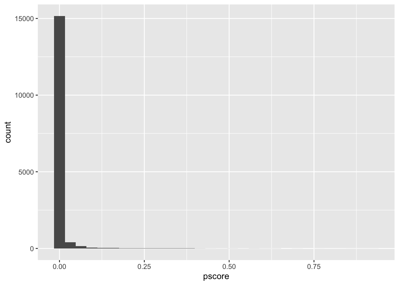
nsw_dw_cpscontrol %>%
  filter(treat == 1) %>%
  ggplot() +
  geom_histogram(aes(x = pscore))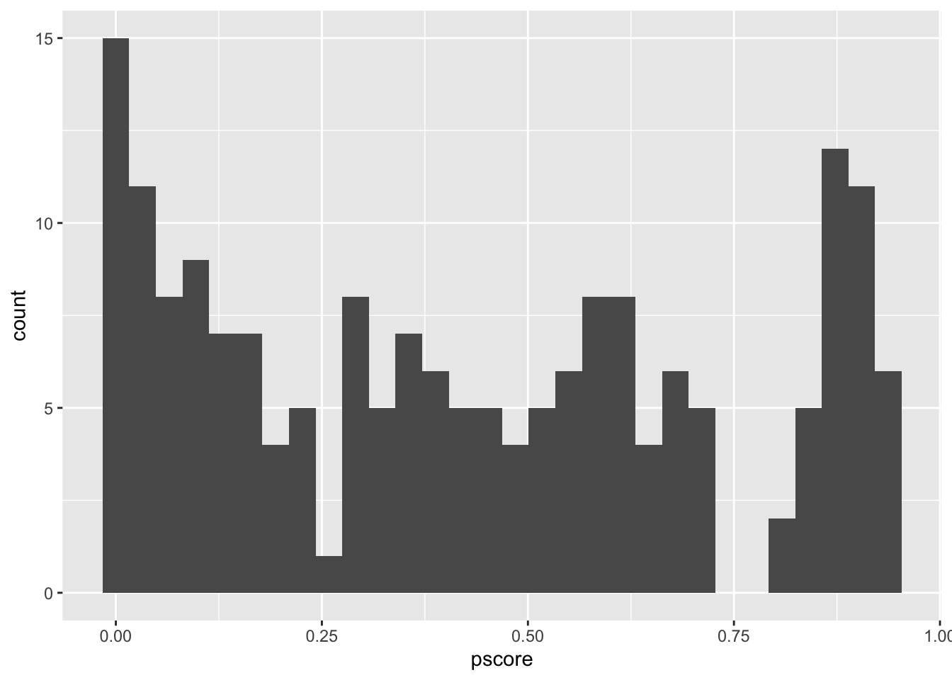
Nearest-neighbor matching with propensity scores
Let’s do a nn matching:
# find matches to the each treated units
m_out <- matchit(treat ~ age + agesq + agecube + educ +
                 educsq + marr + nodegree +
                 black + hisp + re74 + re75 + u74 + u75 + interaction1,
                 data = nsw_dw_cpscontrol, method = "nearest", # specifies that nearest neighbor matching is to be used.
                 distance = "logit", # indicates that the propensity score is estimated using a logistic regression model.
                 ratio =5) # we choose 5 nearest neighbors based on p-score. For each treated unit, five untreated units are selected as matches.
m_data <- match.data(m_out)

# regress Y (re78) on X (treat)
z_out <- zelig(re78 ~ treat +
                 age + agesq + agecube + educ +
               educsq + marr + nodegree +
               black + hisp + re74 + re75 + u74 + u75 + interaction1,
               model = "ls", data = m_data)
## How to cite this model in Zelig:
## R Core Team. 2007.
## ls: Least Squares Regression for Continuous Dependent Variables
## in Christine Choirat, Christopher Gandrud, James Honaker, Kosuke Imai, Gary King, and Olivia Lau,
## "Zelig: Everyone's Statistical Software," https://zeligproject.org/# get predicted outcomes by treatment status
x_out <- setx(z_out, treat = 0)
x1_out <- setx(z_out, treat = 1)
# subtract each unit's matched control from its treatment value, and then divide by N
s_out <- sim(z_out, x = x_out, x1 = x1_out)
summary(s_out)##
## sim x :
## -----
## ev
## mean sd 50% 2.5% 97.5%
## 1 6434.994 220.7491 6428.153 6023.964 6872.491
## pv
## mean sd 50% 2.5% 97.5%
## [1,] 6380.527 6494.469 6362.083 -6161.363 19121.84
##
## sim x1 :
## -----
## ev
## mean sd 50% 2.5% 97.5%
## 1 7876.163 533.8953 7854.445 6802.306 8911.447
## pv
## mean sd 50% 2.5% 97.5%
## [1,] 8285.244 6393.656 8225.047 -4554.956 21336.06
## fd
## mean sd 50% 2.5% 97.5%
## 1 1441.169 599.5709 1416.531 252.5941 2643.903We get ATT of $ ~1440.483 with 95% statistically significance.
Coarsened exact matching
# find matches to the each treated units by coarsening the data
m_out <- matchit(treat ~ age + agesq + agecube + educ +
                   educsq + marr + nodegree +
                   black + hisp + re74 + re75 +
                   u74 + u75 + interaction1,
                 data = nsw_dw_cpscontrol,
                 method = "cem")

# and then we do the same
m_data <- match.data(m_out)

# we may drop the covariates b/c they are already used for matching
m_ate <- lm_robust(re78 ~ treat,
               data = m_data,
               weights = m_data$weights)
m_ate
## Estimate Std. Error t value Pr(>|t|) CI Lower CI Upper DF
## (Intercept) 4098.650 712.1458 5.755352 4.760313e-08 2691.4406 5505.860 149
## treat 2759.926 1187.4090 2.324327 2.145892e-02 413.5906 5106.262 149The treatment effect is around 2759.926 with 95% significance.
PanelMatch: Motivation
Matching has been widely used, but they are mostly used for cross-sectional data. This lab applies a new matching method coupled with difference-in-differences (DiD) estimations. So we have a way of doing matching methods for the analysis of time-series cross-sectional (TSCS) Data. We replicate analyses from Imai et al. (2023)
Load replicated data
load("Acemoglu.RData")Acemoglu et al. (2019) find that democracy promotes economic development. The authors analyse an unbalanced TSCS data set, which consists of a total of 184 countries over a half century from 1960 to 2010.
Codebook
wbcode2: country codes (unit identifier), integeryear: year (time identifier), integery: logged GDP per capita, the dependent variable, numeric; NA = missingunrest: a control variable taking 1 if there is an unrest in a country (represented by wbcode2) during a year (represented by year) and 0 otherwise, numeric; NA = missingdem: the treatment variable, taking 1 if a country (represented by wbcode2) during a year (represented by year) is a democracy and 0 otherwise, numeric; NA = missinglogpop: a control variable multiplied by 100, recording the logged population in a country (represented by wbcode2) during a year (represented by year), numeric; NA = missingPopulationages014oftotal: a control variable recording the percentage of population below age 15 in a country (represented by wbcode2) during a year (represented by year), numeric; NA = missingPopulationages1564oftota: a control variable recording the percentage of population between 15 and 64 in a country (represented by wbcode2) during a year (represented by year), numeric; NA = missingtradewb: a control variable recording the trade volume as a fraction of GDP in a country (represented by wbcode2) during a year (represented by year), numeric; NA = missingnfagdp: a control variable recording the net financial flow as a fraction of GDP in a country (represented by wbcode2) during a year (represented by year), numeric; NA = missingdemoc: an alternative way of coding the treatment variable to be used in conjunction with rever, with explanations in Section A6.3 of Acemoglu et al. (2019), numeric; NA = missingrever: an alternative way of coding the treatment variable to be used in conjunction with rever, with explanations in Section A6.3 of Acemoglu et al. (2019), numeric; NA = missing
Pre-analysis: Visualizing the Treatment Variation Plot
ADis <- DisplayTreatment(unit.id = "wbcode2",
time.id = "year",
xlab = "Year", ylab = "Countries", legend.position = "bottom",
legend.labels = c("Autocracy (Control)", "Democracy (Treatment)"),
title = "Democracy as the Treatment",
treatment = "dem", data = d2)
ADis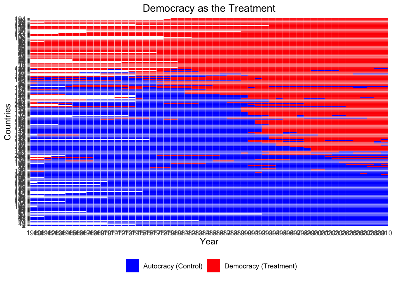 Let’s make it look nicer.
ADis <- DisplayTreatment(unit.id = "wbcode2",
                         time.id = "year",
                         xlab = "Year", ylab = "Countries", legend.position = "bottom",
                         legend.labels = c("Autocracy (Control)", "Democracy (Treatment)"),
                         title = "Democracy as the Treatment",
                         treatment = "dem", data = d2) +
  theme(axis.text.y = element_blank(), axis.ticks.y = element_blank(),
        axis.text.x = element_text(angle=30, size = 6.5, vjust=0.5)) +
  scale_y_discrete(breaks = c(1960, 1970, 1980, 1990, 2000, 2010))
## Scale for y is already present.
## Adding another scale for y, which will replace the existing scale.ADis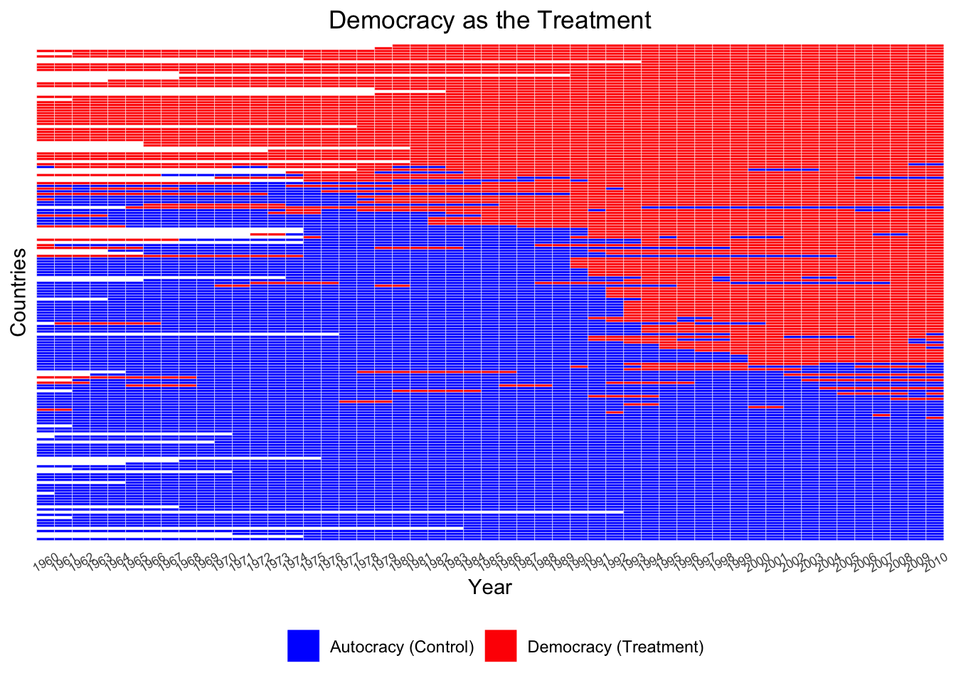
We observe that many countries stayed either democratic or autocratic throughout years with no regime change.
Decide leads and lags values
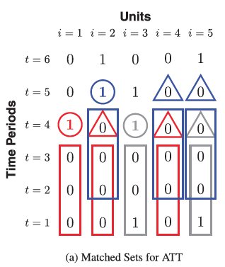
L (lags) determines the matched set of control units that share the identical treatment history from time t − L to t − 1. F (leads) determines the treatment effect on the outcome how many periods after the treatment is administered (short or long term). Imai et al. (2023) said they are theoretical decisions but caution again large values because they reduce the numbers of matches. Let’s say we define L and F both at 4.
Store the covariates formula
formula_Ace <-
  ~ I(lag(y, 1:4)) + I(lag(Populationages014oftotal, 1:4)) +
  I(lag(Populationages1564oftota, 1:4)) + I(lag(unrest, 1:4)) +
  I(lag(tradewb, 1:4)) + I(lag(nfagdp, 1:4)) + I(lag(logpop, 1:4))

formula_Ace_l1 <-
  ~ I(lag(y, 1)) + I(lag(Populationages014oftotal, 1)) +
  I(lag(Populationages1564oftota, 1)) + I(lag(unrest, 1)) +
  I(lag(tradewb, 1)) + I(lag(nfagdp, 1)) + I(lag(logpop, 1))
Construct the Matched Sets
matches_L4_cbps <- PanelMatch(lag = 4, time.id = "year", unit.id = "wbcode2",
                              treatment = "dem", outcome = "y",
                              refinement.method = "mahalanobis", # distance
                              qoi = "ate", # quantity of interest (average treatment effects)
                              data = d2,
                              match.missing = FALSE,
                              covs.formula = formula_Ace, # what covariates to be used for matching
                              size.match = 5, # maximum number of control units that can be included in a matched set.
                              lead = 0:4)
head(matches_L4_cbps$att,20)
## wbcode2 year matched.set.size
## 1 4 1992 74
## 2 4 1997 2
## 3 6 1973 63
## 4 6 1983 73
## 5 7 1991 81
## 6 7 1998 1
## 7 12 1992 74
## 8 13 2003 58
## 9 15 1991 81
## 10 16 1977 63
## 11 17 1991 81
## 12 18 1991 81
## 13 22 1991 81
## 14 25 1982 72
## 15 26 1985 76
## 16 31 1993 65
## 17 34 1990 79
## 18 36 2000 57
## 19 38 1992 74
## 20 40 1990 79matches_L1_cbps <- PanelMatch(lag = 1, time.id = "year", unit.id = "wbcode2",
treatment = "dem", outcome = "y",
refinement.method = "mahalanobis",
qoi = "ate",
data = d2,
match.missing = T,
covs.formula = formula_Ace_l1,
size.match = 5,
lead = 0:4)
head(matches_L1_cbps$att,20)## wbcode2 year matched.set.size
## 1 4 1992 76
## 2 4 1997 63
## 3 6 1973 65
## 4 6 1983 76
## 5 7 1991 82
## 6 7 1998 65
## 7 12 1992 76
## 8 13 2003 62
## 9 15 1991 82
## 10 16 1977 69
## 11 17 1991 82
## 12 18 1991 82
## 13 22 1991 82
## 14 25 1982 77
## 15 26 1985 78
## 16 31 1993 66
## 17 34 1990 81
## 18 36 2000 61
## 19 38 1992 76
## 20 40 1990 81Plot Freq distribution of the number of matched control units
Firs, we extract objects to make histograms with
L4_cbps_att_sizes <- summary(matches_L4_cbps$att)$overview$matched.set.size
L4_cbps_atc_sizes <- summary(matches_L4_cbps$atc)$overview$matched.set.size

L1_cbps_att_sizes <- summary(matches_L1_cbps$att)$overview$matched.set.size
L1_cbps_atc_sizes <- summary(matches_L1_cbps$atc)$overview$matched.set.size
Then, we make the plot.
hist(L4_cbps_att_sizes[L4_cbps_att_sizes>0],
     col = "#ffc6c4", border = NA,
     freq = TRUE,

     breaks = c(1, 5, 10, 15, 20, 25,
                30, 35, 40, 45,
                50, 55, 60, 65, 70, 75, 80,
                85, 90, 95, 100, 105, 110, 115, 120, 125, 130),
     xlim = c(0, 130), ylim= c(0, 30), xlab = "",
     main = "Democratization",
     ylab = "")
lines(x = c(0,0),
      y = c(0, length(L4_cbps_att_sizes[L4_cbps_att_sizes==0])),
      lwd = 4,
      col = "#ffc6c4")

white.hist <- hist(L1_cbps_att_sizes[L1_cbps_att_sizes>0] ,
                   col = rgb(1,1,1,0),

                   breaks = c(1, 5, 10, 15, 20, 25,
                              30, 35, 40, 45,
                              50, 55, 60, 65, 70, 75, 80,
                              85, 90, 95, 100, 105, 110, 115, 120,
                              125, 130),
                   plot = FALSE, lty = 1)
lines(white.hist$breaks, c(0, white.hist$counts),
      type = 'S', lty = 1)
legend(x = 0, y = 30,
       legend = c(paste0("Four Year Lags"),
                  #                         " empty matched sets")
                  paste0("One Year Lag")),

       fill = c("#ffc6c4", "white"),

       xjust = 0,

       pt.cex = 1,
       bty = "n", ncol = 1, cex = 1, bg = "white")

mtext("Frequency", side = 2, line = 2.2, outer=FALSE,
      cex = 0.8)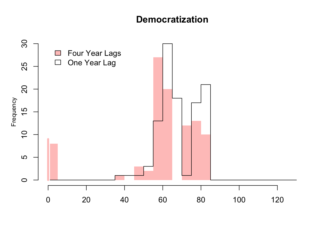
It presents the frequency distribution for the number of matched control units given a treated observation in the case of 1- and 4-year lag as transparent and red bars, respectively. The distribution is presented for the transition from the control to treatment conditions (Democratization: autocracy to democracy). As expected, the number of matched control units generally decreases when we adjust for the treatment history of 4-year period rather than that of 1-year period.
Refine matched sets: Compare different matching methods
Ideally, we want to use the method that maximizes the covariate balance. To refine the matched sets, we apply Mahalanobis distance matching, propensity score matching and propensity score weighting so that we can compare the performance of each refinement method. For matching, we apply up-to-five matching for the Acemoglu et al. study to examine the sensitivity of empirical findings to the maximum number of matches.
matches_L4_mah <- PanelMatch(lag = 4, time.id = "year", unit.id = "wbcode2",
                              treatment = "democ", outcome = "y",
                              refinement.method = "mahalanobis", # distance
                              qoi = "ate", # quantity of interest (average treatment effects)
                              data = d2,
                              match.missing = FALSE,
                              covs.formula = formula_Ace, # what covariates to be used for matching
                              size.match = 5, # maximum number of control units that can be included in a matched set.
                              lead = 0:4)
cov_mah <- get_covariate_balance(matches_L4_mah$att, data = d2, covariates = c("tradewb"), plot = FALSE, ylim = c(-2,2))
# c("Populationages014oftotal","Populationages1564oftota","unrest","tradewb","nfagdp","logpop")
sum(abs(cov_mah))
## [1] 0.6997774matches_L4_psweight <- PanelMatch(lag = 4, time.id = "year", unit.id = "wbcode2",
treatment = "democ", outcome = "y",
refinement.method = "ps.weight",
qoi = "ate", # quantity of interest (average treatment effects)
data = d2,
match.missing = FALSE,
covs.formula = formula_Ace, # what covariates to be used for matching
size.match = 5, # maximum number of control units that can be included in a matched set.
lead = 0:4)
cov_psweight <-get_covariate_balance(matches_L4_psweight$att, data = d2, covariates = c("tradewb"), plot = FALSE, ylim = c(-2,2))
sum(abs(cov_psweight))## [1] 0.8229666matches_L4_psmatch <- PanelMatch(lag = 4, time.id = "year", unit.id = "wbcode2",
treatment = "democ", outcome = "y",
refinement.method = "ps.match",
qoi = "ate", # quantity of interest (average treatment effects)
data = d2,
match.missing = FALSE,
covs.formula = formula_Ace, # what covariates to be used for matching
size.match = 5, # maximum number of control units that can be included in a matched set.
lead = 0:4)
cov_psmatch <- get_covariate_balance(matches_L4_psmatch$att, data = d2, covariates = c("tradewb"), plot = FALSE, ylim = c(-2,2))
sum(abs(cov_psmatch))## [1] 1.21576Use the one that generates the smallest Standardized Mean Difference.
DiD Estimation
We compare the treated and matached (control) units before and after treatment starts.
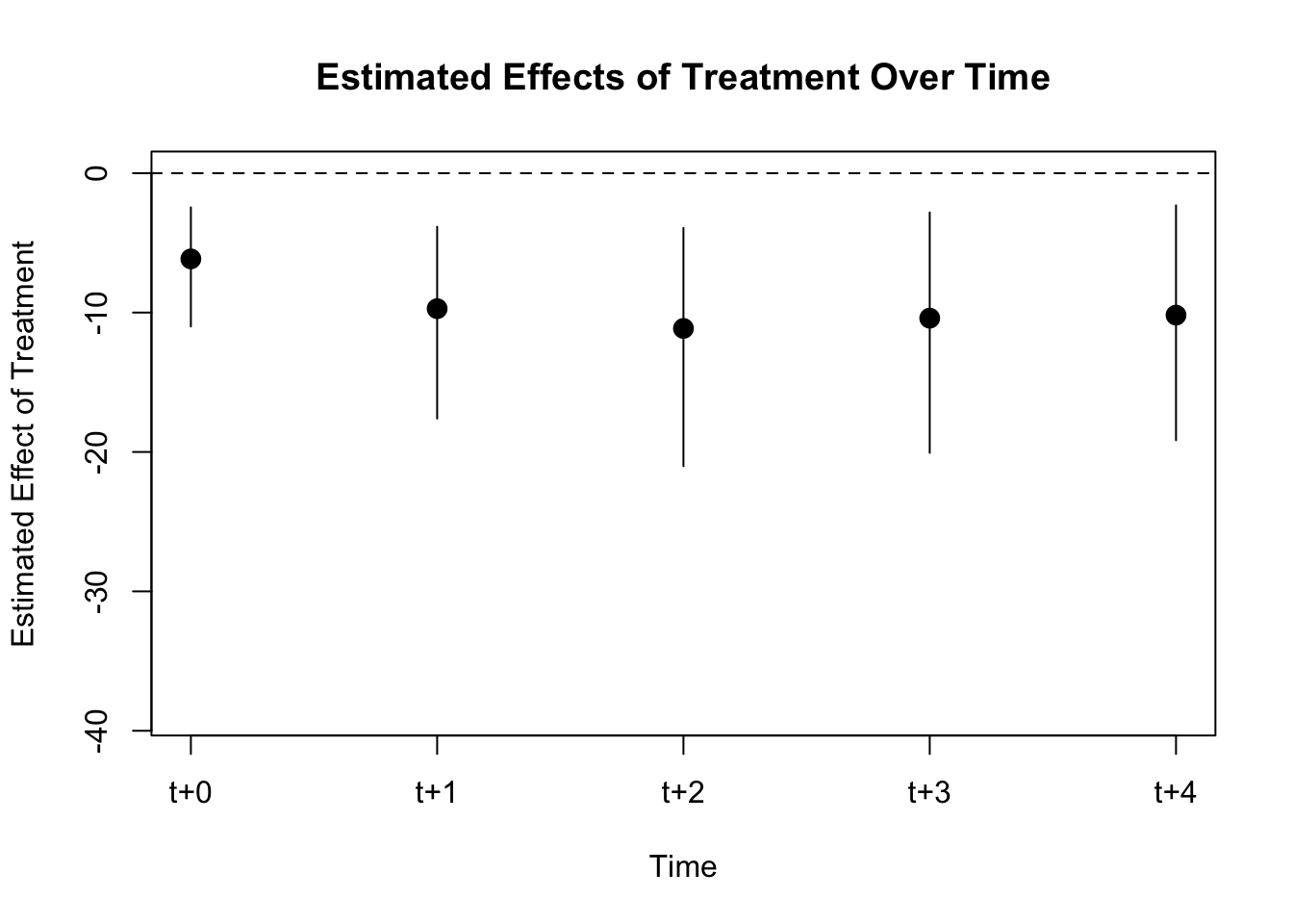
PE.results <- PanelEstimate(sets = matches_L4_mah, data = d2)
summary(PE.results)
## Weighted Difference-in-Differences with Mahalanobis Distance
## Matches created with lags
##
## Standard errors computed with 1000 Weighted bootstrap samples
##
## Estimate of Average Treatment Effect (ATE) by Period:## $summary
## estimate std.error 2.5% 97.5%
## t+0 -1.217017 0.6551383 -2.428151 0.1287337
## t+1 -1.781383 1.2257035 -3.979640 0.8376445
## t+2 -1.932438 1.6553463 -4.899568 1.6978761
## t+3 -1.768251 2.2632663 -5.797491 3.1190259
## t+4 -1.979402 2.5947703 -6.544133 3.6071232
##
## $lag
## [1] 4
##
## $iterations
## [1] 1000
##
## $qoi
## [1] "ate"plot(PE.results)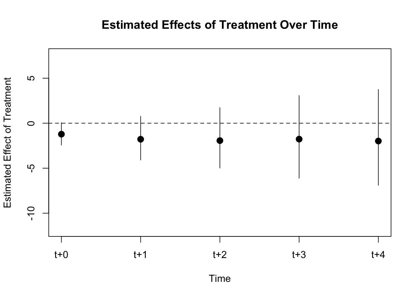
We observe no effect of democracy on gdp growth.
